Семи-эмпирические вычисления: Mopac
In [1]:
import pybel
from os import system
from IPython.display import display, Image
import pandas as pd
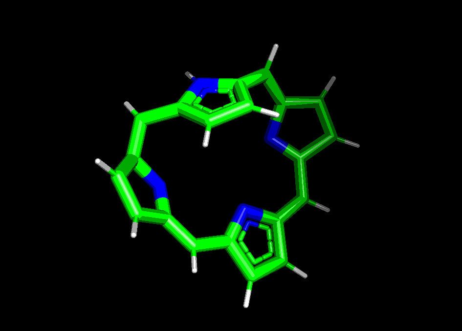
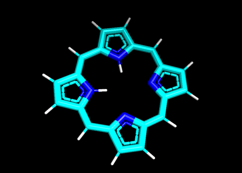
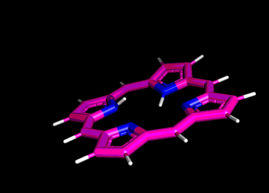
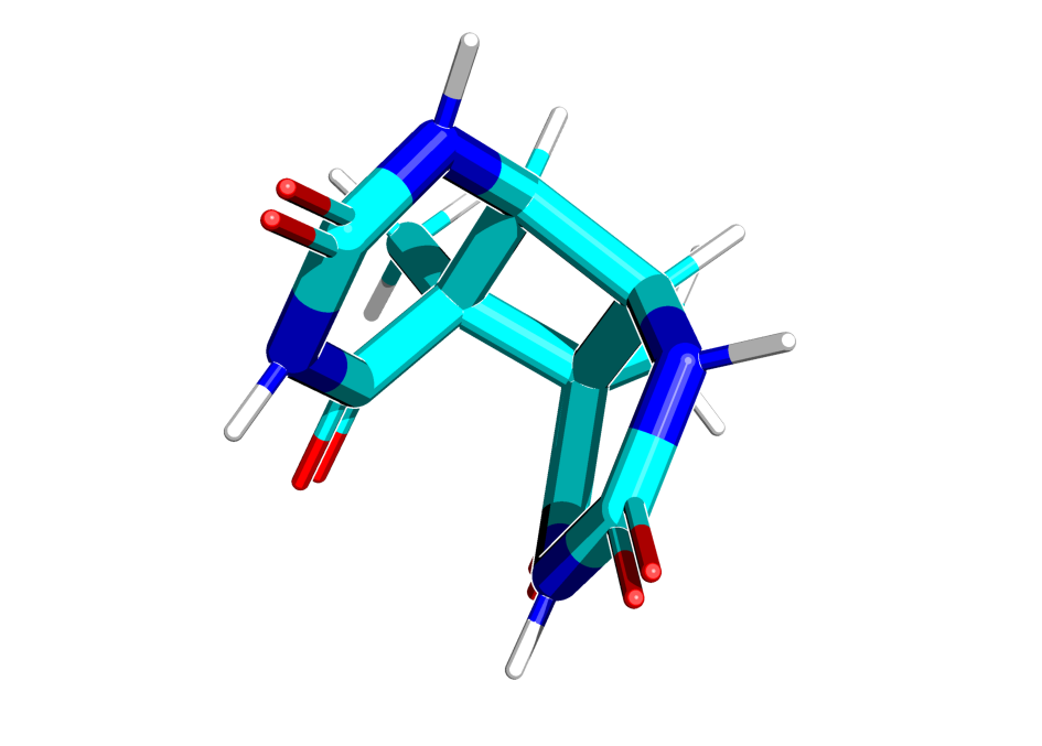
Сравним структуры порфирина, полученные pybel и двумя способами в Mopac:
In [2]:
def run_mopac(mol, name, param='PM6', syscharge=None):
    if (type(syscharge) == str):
        charge = syscharge
    else:
        charge = mol.charge

    system("export MOPAC_LICENSE='/home/preps/golovin/progs/mopac/'")
    mop = mol.write(format='mopin', filename='%s.mop' % name, \
                   opt={'k':'%s CHARGE=%s' % (param, charge)}, \
                   overwrite=True)

    system("echo | /home/preps/golovin/progs/mopac/MOPAC2016.exe %s.mop" % name)
    opt=pybel.readfile('mopout','%s.out' % name)
    for i in opt:
        i.write(format='pdb',filename='%s.pdb' % name, overwrite=True)
Сгенерируем структуру порфирина при помощи babel:
In [3]:
mol=pybel.readstring('smi','C1=CC2=CC3=CC=C(N3)C=C4C=CC(=N4)C=C5C=CC(=N5)C=C1N2')
mol.addh()
mol.make3D(steps=500)
mol.write(format="pdb", filename='porph_pybl.pdb', overwrite=True)
mol
Out[3]:
In [10]:
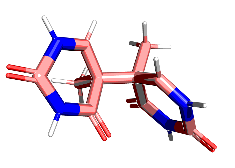
run_mopac(mol, 'porph_pm6', param='PM6')
In [11]:
run_mopac(mol, 'porph_am1', param='AM1')
Теперь рассчитаем возбужденные состояния порфирина:
In [24]:
%%bash
cp porph_pm6.mop porph_pm6_ex.mop
echo '' >> porph_pm6_ex.mop
echo 'cis c.i.=4 meci oldgeo' >> porph_pm6_ex.mop
echo 'some description' >> porph_pm6_ex.mop
In [ ]:
%%bash
export MOPAC_LICENSE='/home/preps/golovin/progs/mopac/'
nohup echo | /home/preps/golovin/progs/mopac/MOPAC2016.exe porph_pm6_ex.mop > log.log&
In [25]:
with open('porph_pm6_ex.out', 'r') as f:
    lines = f.readlines()
ev = []
i, j = 0, 0
while (i < len(lines)):
    if ("RELATIVE" in lines[i]):
        j = 1
        i += 1
    elif ("The \"+\" symbol indicates the root used" in lines[i]):
        j = 0
    if (j) and (lines[i] != '\n'):
        ev.append(float(lines[i].split()[1]))
    i+=1
ev = ev[1:]
Зная энергию каждого из состояний, можем посчитать длины волн (в нанометрах), при котором происходят соотвествующие им переходы.
In [39]:
states = pd.DataFrame(data={'lambdas':[1239.84193/item for item in ev], 'energies':ev}, \
                   index=range(2, 10))
states
Out[39]:
| energies | lambdas | |
|---|---|---|
| 2 | 1.766016 | 702.055887 |
| 3 | 2.171129 | 571.058620 |
| 4 | 2.327297 | 532.739023 |
| 5 | 2.694206 | 460.188245 |
| 6 | 3.091973 | 400.987308 |
| 7 | 3.144006 | 394.351006 |
| 8 | 3.756254 | 330.074039 |
| 9 | 3.765039 | 329.303874 |
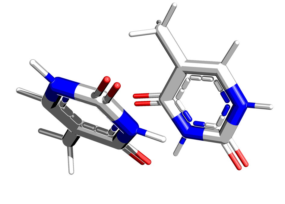
Попробуем смоделировать переход тиминового димера в тимины при возбуждении системы:
In [44]:
! wget http://kodomo.fbb.msu.ru/FBB/year_08/term6/td.pdb
--2018-03-28 18:29:49--  http://kodomo.fbb.msu.ru/FBB/year_08/term6/td.pdb
Resolving kodomo.fbb.msu.ru... 192.168.180.1
Connecting to kodomo.fbb.msu.ru|192.168.180.1|:80... connected.
HTTP request sent, awaiting response... 200 OK
Length: 2010 (2.0K) [chemical/x-pdb]
Saving to: `td.pdb'

100%[======================================>] 2,010       --.-K/s   in 0s

2018-03-28 18:29:49 (247 MB/s) - `td.pdb' saved [2010/2010]
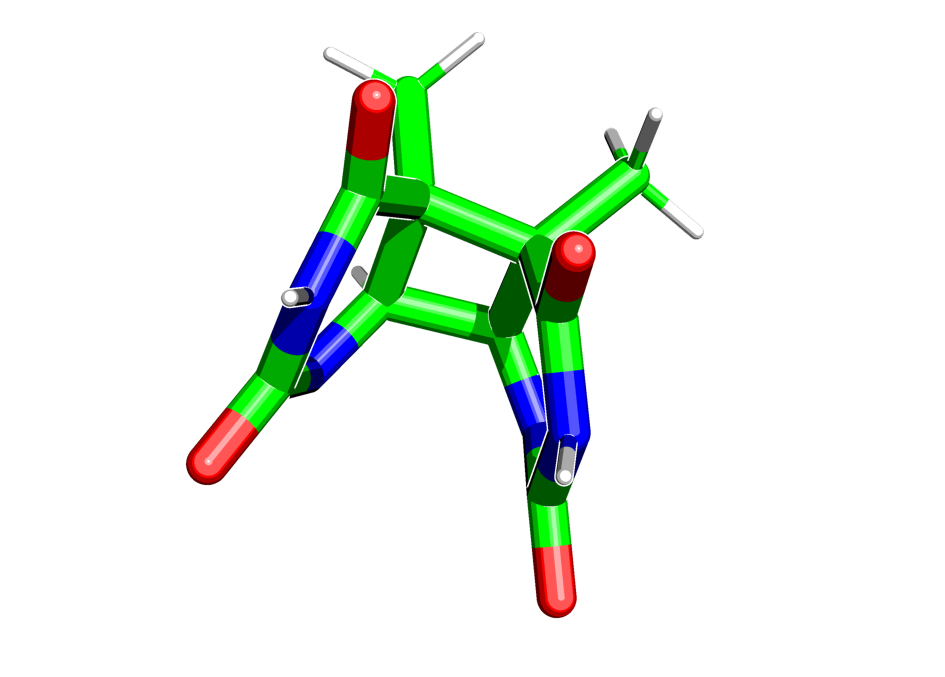
In [56]:
td_0 = pybel.readfile("pdb", "td.pdb").next()
run_mopac(td_0, "td_1", param='PM6', syscharge='0')
In [57]:
td_1 = pybel.readfile("pdb", "td_1.pdb").next()
run_mopac(td_1, "td_2", param='PM6', syscharge='+2')
In [58]:
td_2 = pybel.readfile("pdb", "td_2.pdb").next()
run_mopac(td_2, "td_3", param='PM6', syscharge='0')
In [60]:
%%bash
grep "TOTAL ENERGY" td_*.out >> td.log
In [74]:
with open("td.log", "r") as f:
    for num, val in enumerate(f):
        print "State %s " % str(num+1), val.split()[-2], "EV"
State 1  -3273.57685 EV
State 2  -3253.90536 EV
State 3  -3273.78789 EV
Максимум энергии соответствует ионизированному интермедиату, а состояния димера и двух мономеров почти эквивалентны, при этом состояние двух мономеров чуть более выгодное. Система "свалилась" в него как в наилучше после того, как мы сообщилои ей достаточное количество энергии.
Ab initio вычисления: Orca
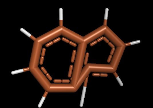
Будем искать оптимальную геометрию нафталена и азулена и рассчитаем теплоты их образования.
К сожалению, pybel оказался абсолютно неспособен сделать 3D-молекулу нафталина методом make3D(), какие бы силовые поля и количество шагов оптимизации я не применял. получалось нечто такое (см. рис. 8), и при последующей оптимизации мопаком данная пародия на молекулу конечно же скатывалась в азулен. Поэтому я создал .mol-файлы с помощью самого бабеля:
In [3]:
%%bash
echo "c1ccc2ccccc2c1" > nph.smi
echo "C1=CC=C2C=CC=C2C=C1" > azu.smi
obgen nph.smi > NPH.mol
obgen azu.smi > AZU.mol
A T O M   T Y P E S

IDX	TYPE	RING
1	37	AR
2	37	AR
3	37	AR
4	37	AR
5	37	AR
6	37	AR
7	37	AR
8	37	AR
9	37	AR
10	37	AR
11	5	NO
12	5	NO
13	5	NO
14	5	NO
15	5	NO
16	5	NO
17	5	NO
18	5	NO

F O R M A L   C H A R G E S

IDX	CHARGE
1	0.000000
2	0.000000
3	0.000000
4	0.000000
5	0.000000
6	0.000000
7	0.000000
8	0.000000
9	0.000000
10	0.000000
11	0.000000
12	0.000000
13	0.000000
14	0.000000
15	0.000000
16	0.000000
17	0.000000
18	0.000000

P A R T I A L   C H A R G E S

IDX	CHARGE
1	-0.150000
2	-0.150000
3	-0.150000
4	0.000000
5	-0.150000
6	-0.150000
7	-0.150000
8	-0.150000
9	0.000000
10	-0.150000
11	0.150000
12	0.150000
13	0.150000
14	0.150000
15	0.150000
16	0.150000
17	0.150000
18	0.150000

S E T T I N G   U P   C A L C U L A T I O N S

SETTING UP BOND CALCULATIONS...
SETTING UP ANGLE & STRETCH-BEND CALCULATIONS...
SETTING UP TORSION CALCULATIONS...
SETTING UP OOP CALCULATIONS...
SETTING UP VAN DER WAALS CALCULATIONS...
SETTING UP ELECTROSTATIC CALCULATIONS...

S T E E P E S T   D E S C E N T

STEPS = 500

STEP n       E(n)         E(n-1)
------------------------------------
    0      78.012      ----
   10    45.34567    46.18691
   20    39.76726    40.17474
   30    36.72344    36.95794
   40    34.93471    35.07511
   50    33.84158    33.92931
   60    33.14119    33.19883
   70    32.66892    32.70873
   80    32.33485    32.36361
   90    32.08878    32.11032
  100    31.90167    31.91826
  110    31.75597    31.76901
  120    31.64055    31.65094
  130    31.54797    31.55635
  140    31.47308    31.47988
  150    31.41214    31.41769
  160    31.36235    31.36689
  170    31.32155    31.32527
  180    31.28805    31.29111
  190    31.26052    31.26304
  200    31.23788    31.23995
  210    31.21925    31.22095
  220    31.20391    31.20531
  230    31.19129    31.19244
  240    31.18090    31.18185
  250    31.17236    31.17314
  260    31.16532    31.16597
  270    31.15954    31.16007
  280    31.15478    31.15521
  290    31.15087    31.15123
  300    31.14765    31.14794
  310    31.14501    31.14525
  320    31.14284    31.14304
  330    31.14105    31.14122
  340    31.13959    31.13972
  350    31.13838    31.13849
  360    31.13739    31.13748
  370    31.13658    31.13665
  380    31.13591    31.13597
  390    31.13536    31.13541
  400    31.13491    31.13495
  410    31.13454    31.13457
  420    31.13423    31.13426
  430    31.13398    31.13400
  440    31.13378    31.13380
  450    31.13361    31.13362
  460    31.13347    31.13348
  470    31.13336    31.13337
  480    31.13326    31.13327
  490    31.13319    31.13319
  500    31.13312    31.13313

W E I G H T E D   R O T O R   S E A R C H

  NUMBER OF ROTATABLE BONDS: 0
  NUMBER OF POSSIBLE ROTAMERS: 1
  GENERATED ONLY ONE CONFORMER


S T E E P E S T   D E S C E N T

STEPS = 500

STEP n       E(n)         E(n-1)
------------------------------------
    0      31.133      ----
   10    31.13285    31.13285
   20    31.13285    31.13285
   30    31.13285    31.13285
   40    31.13285    31.13285
   50    31.13284    31.13284
   60    31.13284    31.13284
   70    31.13284    31.13284
   80    31.13284    31.13284
   90    31.13284    31.13284
  100    31.13284    31.13284
  110    31.13284    31.13284
  120    31.13284    31.13284
  130    31.13284    31.13284
  140    31.13284    31.13284
  150    31.13284    31.13284
  160    31.13284    31.13284
  170    31.13284    31.13284
  180    31.13284    31.13284
  190    31.13284    31.13284
  200    31.13284    31.13284
  210    31.13284    31.13284
  220    31.13284    31.13284
  230    31.13284    31.13284
  240    31.13284    31.13284
  250    31.13284    31.13284
  260    31.13284    31.13284
  270    31.13284    31.13284
  280    31.13284    31.13284
  290    31.13284    31.13284
  300    31.13284    31.13284
  310    31.13284    31.13284
  320    31.13284    31.13284
  330    31.13284    31.13284
  340    31.13284    31.13284
  350    31.13284    31.13284
  360    31.13284    31.13284
  370    31.13284    31.13284
  380    31.13284    31.13284
  390    31.13284    31.13284
  400    31.13284    31.13284
  410    31.13284    31.13284
  420    31.13284    31.13284
  430    31.13284    31.13284
  440    31.13284    31.13284
  450    31.13284    31.13284
  460    31.13284    31.13284
  470    31.13284    31.13284
  480    31.13284    31.13284
  490    31.13284    31.13284
  500    31.13284    31.13284

A T O M   T Y P E S

IDX	TYPE	RING
1	2	AL
2	2	AL
3	2	AL
4	2	AL
5	2	AL
6	2	AL
7	2	AL
8	2	AL
9	2	AL
10	2	AL
11	5	NO
12	5	NO
13	5	NO
14	5	NO
15	5	NO
16	5	NO
17	5	NO
18	5	NO

F O R M A L   C H A R G E S

IDX	CHARGE
1	0.000000
2	0.000000
3	0.000000
4	0.000000
5	0.000000
6	0.000000
7	0.000000
8	0.000000
9	0.000000
10	0.000000
11	0.000000
12	0.000000
13	0.000000
14	0.000000
15	0.000000
16	0.000000
17	0.000000
18	0.000000

P A R T I A L   C H A R G E S

IDX	CHARGE
1	-0.150000
2	-0.150000
3	-0.150000
4	0.000000
5	-0.150000
6	-0.150000
7	-0.150000
8	0.000000
9	-0.150000
10	-0.150000
11	0.150000
12	0.150000
13	0.150000
14	0.150000
15	0.150000
16	0.150000
17	0.150000
18	0.150000

S E T T I N G   U P   C A L C U L A T I O N S

SETTING UP BOND CALCULATIONS...
SETTING UP ANGLE & STRETCH-BEND CALCULATIONS...
SETTING UP TORSION CALCULATIONS...
SETTING UP OOP CALCULATIONS...
SETTING UP VAN DER WAALS CALCULATIONS...
SETTING UP ELECTROSTATIC CALCULATIONS...

S T E E P E S T   D E S C E N T

STEPS = 500

STEP n       E(n)         E(n-1)
------------------------------------
    0    133874.429      ----
   10    834.20427    926.42373
   20    403.78175    419.99579
   30    312.02255    316.41715
   40    280.14326    282.68585
   50    253.75745    258.72647
   60    130.30627    133.31758
   70    108.41814    109.97920
   80    98.38194    99.02508
   90    94.07032    94.37443
  100    91.81845    91.99663
  110    90.34916    90.47825
  120    89.17490    89.28720
  130    88.06398    88.17763
  140    86.85413    86.98507
  150    85.36118    85.53111
  160    83.28879    83.53580
  170    80.08544    80.48068
  180    74.83729    75.47850
  190    67.11526    67.95882
  200    58.83594    59.58563
  210    52.90038    53.35552
  220    49.64417    49.87773
  230    48.01930    48.13449
  240    47.21420    47.27201
  250    46.80055    46.83109
  260    46.57405    46.59140
  270    46.43990    46.45059
  280    46.35381    46.36092
  290    46.29438    46.29944
  300    46.25075    46.25456
  310    46.21705    46.22005
  320    46.18992    46.19238
  330    46.16730    46.16938
  340    46.14787    46.14968
  350    46.13074    46.13236
  360    46.11528    46.11675
  370    46.10100    46.10237
  380    46.08754    46.08884
  390    46.07460    46.07586
  400    46.06190    46.06315
  410    46.04918    46.05045
  420    46.03619    46.03749
  430    46.02261    46.02398
  440    46.00808    46.00957
  450    45.99214    45.99379
  460    45.97414    45.97602
  470    45.95318    45.95540
  480    45.92806    45.93070
  490    45.92100    45.92141
  500    45.91684    45.91726

W E I G H T E D   R O T O R   S E A R C H

  NUMBER OF ROTATABLE BONDS: 0
  NUMBER OF POSSIBLE ROTAMERS: 1
  GENERATED ONLY ONE CONFORMER


S T E E P E S T   D E S C E N T

STEPS = 500

STEP n       E(n)         E(n-1)
------------------------------------
    0      45.881      ----
   10    45.87775    45.87802
   20    45.87514    45.87539
   30    45.87269    45.87293
   40    45.87039    45.87061
   50    45.86821    45.86842
   60    45.86614    45.86634
   70    45.86415    45.86434
   80    45.86223    45.86242
   90    45.86037    45.86055
  100    45.85856    45.85874
  110    45.85679    45.85696
  120    45.85504    45.85521
  130    45.85332    45.85349
  140    45.85161    45.85178
  150    45.84991    45.85008
  160    45.84820    45.84837
  170    45.84649    45.84666
  180    45.84476    45.84494
  190    45.84301    45.84319
  200    45.84123    45.84141
  210    45.83942    45.83960
  220    45.83756    45.83774
  230    45.83564    45.83584
  240    45.83367    45.83387
  250    45.83163    45.83183
  260    45.82950    45.82972
  270    45.82730    45.82752
  280    45.82500    45.82523
  290    45.82260    45.82284
  300    45.82010    45.82035
  310    45.81772    45.81787
  320    45.81709    45.81715
  330    45.81649    45.81655
  340    45.81590    45.81595
  350    45.81530    45.81536
  360    45.81472    45.81478
  370    45.81413    45.81419
  380    45.81355    45.81361
  390    45.81297    45.81302
  400    45.81238    45.81244
  410    45.81180    45.81186
  420    45.81122    45.81128
  430    45.81064    45.81069
  440    45.81005    45.81011
  450    45.80947    45.80953
  460    45.80888    45.80894
  470    45.80830    45.80836
  480    45.80771    45.80777
  490    45.80713    45.80719
  500    45.80654    45.80660
In [6]:
nph = pybel.readfile('sdf', 'NPH.mol').next()
nph
Out[6]:
In [4]:
azu = pybel.readfile('sdf', 'AZU.mol').next()
azu
Out[4]:
In [7]:
def prep_orca(mol, name):
    run_mopac(mol, name, param='PM6')
    opt = pybel.readfile('pdb', '%s.pdb' % name).next()
    headers = ["!HF RHF 6-31G", "!DFT RHF 6-31G"]
    for i in range(len(headers)):
        mask = headers[i].split(' ')[0][1:]
        opt.write(format='orcainp', opt={'k':headers[i]}, \
                 filename='%s_%s.oinp' % (name, mask), \
                 overwrite=True)
        with open('%s_%s.oinp' % (name, mask), 'r') as f:
            lines = f.readlines()
        with open('%s_%s.oinp' % (name, mask), 'w') as f:
            for line in lines:
                if ('! insert inline commands here' in line):
                    line = headers[i] + '\n'
                f.write(line)
In [8]:
prep_orca(azu, 'azu')
In [9]:
prep_orca(nph, 'nph')
Отлично! теперь запустим орку:
In [12]:
%%bash
/srv/databases/orca/orca azu_DFT.oinp | tee azu_DFT_opt.log
*****************
* O R C A *
*****************
--- An Ab Initio, DFT and Semiempirical electronic structure package ---
#######################################################
# -***- #
# Department of molecular theory and spectroscopy #
# Directorship: Frank Neese #
# Max Planck Institute for Chemical Energy Conversion #
# D-45470 Muelheim/Ruhr #
# Germany #
# #
# All rights reserved #
# -***- #
#######################################################
Program Version 3.0.3 - RELEASE -
With contributions from (in alphabetic order):
Ute Becker : Parallelization
Dmytro Bykov : SCF Hessian
Dmitry Ganyushin : Spin-Orbit,Spin-Spin,Magnetic field MRCI
Andreas Hansen : Spin unrestricted coupled pair/coupled cluster methods
Dimitrios Liakos : Extrapolation schemes; parallel MDCI
Robert Izsak : Overlap fitted RIJCOSX, COSX-SCS-MP3
Christian Kollmar : KDIIS, OOCD, Brueckner-CCSD(T), CCSD density
Simone Kossmann : Meta GGA functionals, TD-DFT gradient, OOMP2, MP2 Hessian
Taras Petrenko : DFT Hessian,TD-DFT gradient, ASA and ECA modules, normal mode analysis, Resonance Raman, ABS, FL, XAS/XES, NRVS
Christoph Reimann : Effective Core Potentials
Michael Roemelt : Restricted open shell CIS
Christoph Riplinger : Improved optimizer, TS searches, QM/MM, DLPNO-CCSD
Barbara Sandhoefer : DKH picture change effects
Igor Schapiro : Molecular dynamics
Kantharuban Sivalingam : CASSCF convergence, NEVPT2
Boris Wezisla : Elementary symmetry handling
Frank Wennmohs : Technical directorship
We gratefully acknowledge several colleagues who have allowed us to
interface, adapt or use parts of their codes:
Stefan Grimme, W. Hujo, H. Kruse, T. Risthaus : VdW corrections, initial TS optimization,
DFT functionals, gCP
Ed Valeev : LibInt (2-el integral package), F12 methods
Garnet Chan, S. Sharma, R. Olivares : DMRG
Ulf Ekstrom : XCFun DFT Library
Mihaly Kallay : mrcc (arbitrary order and MRCC methods)
Andreas Klamt, Michael Diedenhofen : otool_cosmo (COSMO solvation model)
Frank Weinhold : gennbo (NPA and NBO analysis)
Christopher J. Cramer and Donald G. Truhlar : smd solvation model
Your calculation uses the libint2 library for the computation of 2-el integrals
For citations please refer to: http://libint.valeyev.net
This ORCA versions uses:
CBLAS interface : Fast vector & matrix operations
LAPACKE interface : Fast linear algebra routines
SCALAPACK package : Parallel linear algebra routines
Your calculation utilizes the basis: 6-31G
Cite in your paper:
H - He: W.J. Hehre, R. Ditchfield and J.A. Pople, J. Chem. Phys. 56,
Li - Ne: 2257 (1972). Note: Li and B come from J.D. Dill and J.A.
Pople, J. Chem. Phys. 62, 2921 (1975).
Na - Ar: M.M. Francl, W.J. Pietro, W.J. Hehre, J.S. Binkley, M.S. Gordon,
D.J. DeFrees and J.A. Pople, J. Chem. Phys. 77, 3654 (1982)
K - Zn: V. Rassolov, J.A. Pople, M. Ratner and T.L. Windus, J. Chem. Phys.
(accepted, 1998)
Note: He and Ne are unpublished basis sets taken from the Gaussian program
================================================================================
WARNINGS
Please study these warnings very carefully!
================================================================================
Now building the actual basis set
INFO : the flag for use of LIBINT has been found!
================================================================================
INPUT FILE
================================================================================
NAME = azu_DFT.oinp
| 1> # ORCA input file
| 2> # azu.pdb
| 3> !DFT RHF 6-31G
| 4> * xyz 0 1
| 5> C -0.12000 -0.14700 -0.34100
| 6> C 1.23500 -0.14700 -0.34100
| 7> C 2.13700 0.97100 -0.34100
| 8> C 1.82600 2.28600 -0.35200
| 9> C 2.80600 3.38700 -0.36300
| 10> C 2.12900 4.57200 -0.38700
| 11> C 0.69500 4.30900 -0.38600
| 12> C 0.48900 2.94900 -0.36300
| 13> C -0.78300 2.28800 -0.35100
| 14> C -1.04000 0.95900 -0.34200
| 15> H -0.62000 -1.12900 -0.33900
| 16> H 1.74000 -1.12400 -0.33800
| 17> H 3.20300 0.69700 -0.33300
| 18> H 3.86700 3.23300 -0.35400
| 19> H 2.54600 5.56300 -0.40300
| 20> H -0.04900 5.08100 -0.40100
| 21> H -1.64300 2.97600 -0.34900
| 22> H -2.09600 0.65300 -0.33400
| 23> *
| 24>
| 25> ****END OF INPUT****
================================================================================
****************************
* Single Point Calculation *
****************************
---------------------------------
CARTESIAN COORDINATES (ANGSTROEM)
---------------------------------
C -0.120000 -0.147000 -0.341000
C 1.235000 -0.147000 -0.341000
C 2.137000 0.971000 -0.341000
C 1.826000 2.286000 -0.352000
C 2.806000 3.387000 -0.363000
C 2.129000 4.572000 -0.387000
C 0.695000 4.309000 -0.386000
C 0.489000 2.949000 -0.363000
C -0.783000 2.288000 -0.351000
C -1.040000 0.959000 -0.342000
H -0.620000 -1.129000 -0.339000
H 1.740000 -1.124000 -0.338000
H 3.203000 0.697000 -0.333000
H 3.867000 3.233000 -0.354000
H 2.546000 5.563000 -0.403000
H -0.049000 5.081000 -0.401000
H -1.643000 2.976000 -0.349000
H -2.096000 0.653000 -0.334000
----------------------------
CARTESIAN COORDINATES (A.U.)
----------------------------
NO LB ZA FRAG MASS X Y Z
0 C 6.0000 0 12.011 -0.226767136070550 -0.277789741686424 -0.644396611667147
1 C 6.0000 0 12.011 2.333811775392746 -0.277789741686424 -0.644396611667147
2 C 6.0000 0 12.011 4.038344748189715 1.834924076037535 -0.644396611667147
3 C 6.0000 0 12.011 3.450639920540206 4.319913942143981 -0.665183599140281
4 C 6.0000 0 12.011 5.302571531783032 6.400502415591279 -0.685970586613414
5 C 6.0000 0 12.011 4.023226939118345 8.639827884287962 -0.731324013827524
6 C 6.0000 0 12.011 1.313359663075270 8.142829911066674 -0.729434287693603
7 C 6.0000 0 12.011 0.924076079487492 5.572802368933771 -0.685970586613414
8 C 6.0000 0 12.011 -1.479655562860340 4.323693394411824 -0.663293873006359
9 C 6.0000 0 12.011 -1.965315179278102 1.812247362430480 -0.646286337801068
10 H 1.0000 0 1.008 -1.171630203031176 -2.133500805197093 -0.640617159399304
11 H 1.0000 0 1.008 3.288123473022978 -2.124052174527487 -0.638727433265383
12 H 1.0000 0 1.008 6.052792806949769 1.317139115343112 -0.629278802595777
13 H 1.0000 0 1.008 7.307570959873480 6.109484590967407 -0.668963051408123
14 H 1.0000 0 1.008 4.811242736963506 10.512546483003922 -0.761559631970264
15 H 1.0000 0 1.008 -0.092596580562141 9.601698486453881 -0.757780179702422
16 H 1.0000 0 1.008 -3.104820038032616 5.623824974549644 -0.659514420738517
17 H 1.0000 0 1.008 -3.960865976698944 1.233991165450577 -0.631168528729698
--------------------------------
INTERNAL COORDINATES (ANGSTROEM)
--------------------------------
C 0 0 0 0.000000 0.000 0.000
C 1 0 0 1.355000 0.000 0.000
C 2 1 0 1.436499 128.897 0.000
C 3 2 1 1.351320 127.796 359.410
C 4 3 2 1.474016 125.023 180.557
C 5 4 3 1.364965 108.592 179.351
C 6 5 4 1.457918 109.343 0.283
C 7 6 5 1.375705 109.004 359.918
C 8 7 6 1.433544 126.075 179.816
C 9 8 7 1.353651 128.405 179.270
H 1 2 3 1.101966 116.984 180.117
H 2 1 3 1.099801 117.334 179.824
H 3 2 1 1.100680 114.481 179.542
H 5 4 3 1.072156 123.407 359.412
H 6 5 4 1.075279 127.447 180.190
H 7 6 5 1.072262 123.545 179.906
H 9 8 7 1.101339 113.881 359.263
H 10 9 8 1.099471 117.107 180.037
---------------------------
INTERNAL COORDINATES (A.U.)
---------------------------
C 0 0 0 0.000000 0.000 0.000
C 1 0 0 2.560579 0.000 0.000
C 2 1 0 2.714589 128.897 0.000
C 3 2 1 2.553626 127.796 359.410
C 4 3 2 2.785486 125.023 180.557
C 5 4 3 2.579410 108.592 179.351
C 6 5 4 2.755066 109.343 0.283
C 7 6 5 2.599706 109.004 359.918
C 8 7 6 2.709006 126.075 179.816
C 9 8 7 2.558030 128.405 179.270
H 1 2 3 2.082413 116.984 180.117
H 2 1 3 2.078323 117.334 179.824
H 3 2 1 2.079983 114.481 179.542
H 5 4 3 2.026081 123.407 359.412
H 6 5 4 2.031984 127.447 180.190
H 7 6 5 2.026281 123.545 179.906
H 9 8 7 2.081229 113.881 359.263
H 10 9 8 2.077699 117.107 180.037
---------------------
BASIS SET INFORMATION
---------------------
There are 2 groups of distinct atoms
Group 1 Type C : 10s4p contracted to 3s2p pattern {631/31}
Group 2 Type H : 4s contracted to 2s pattern {31}
Atom 0C basis set group => 1
Atom 1C basis set group => 1
Atom 2C basis set group => 1
Atom 3C basis set group => 1
Atom 4C basis set group => 1
Atom 5C basis set group => 1
Atom 6C basis set group => 1
Atom 7C basis set group => 1
Atom 8C basis set group => 1
Atom 9C basis set group => 1
Atom 10H basis set group => 2
Atom 11H basis set group => 2
Atom 12H basis set group => 2
Atom 13H basis set group => 2
Atom 14H basis set group => 2
Atom 15H basis set group => 2
Atom 16H basis set group => 2
Atom 17H basis set group => 2
------------------------------------------------------------------------------
ORCA GTO INTEGRAL CALCULATION
------------------------------------------------------------------------------
BASIS SET STATISTICS AND STARTUP INFO
# of primitive gaussian shells ... 172
# of primitive gaussian functions ... 252
# of contracted shell ... 66
# of contracted basis functions ... 106
Highest angular momentum ... 1
Maximum contraction depth ... 6
Integral package used ... LIBINT
Integral threshhold Thresh ... 1.000e-10
Primitive cut-off TCut ... 1.000e-11
INTEGRAL EVALUATION
One electron integrals ... done
Pre-screening matrix ... done
Shell pair data ... done ( 0.003 sec)
-------------------------------------------------------------------------------
ORCA SCF
-------------------------------------------------------------------------------
------------
SCF SETTINGS
------------
Hamiltonian:
Density Functional Method .... DFT(GTOs)
Exchange Functional Exchange .... Slater
X-Alpha parameter XAlpha .... 0.666667
Correlation Functional Correlation .... VWN-5
Gradients option PostSCFGGA .... off
General Settings:
Integral files IntName .... azu_DFT.oinp
Hartree-Fock type HFTyp .... RHF
Total Charge Charge .... 0
Multiplicity Mult .... 1
Number of Electrons NEL .... 68
Basis Dimension Dim .... 106
Nuclear Repulsion ENuc .... 452.5419020564 Eh
Convergence Acceleration:
DIIS CNVDIIS .... on
Start iteration DIISMaxIt .... 12
Startup error DIISStart .... 0.200000
# of expansion vecs DIISMaxEq .... 5
Bias factor DIISBfac .... 1.050
Max. coefficient DIISMaxC .... 10.000
Newton-Raphson CNVNR .... off
SOSCF CNVSOSCF .... on
Start iteration SOSCFMaxIt .... 150
Startup grad/error SOSCFStart .... 0.003300
Level Shifting CNVShift .... on
Level shift para. LevelShift .... 0.2500
Turn off err/grad. ShiftErr .... 0.0010
Zerner damping CNVZerner .... off
Static damping CNVDamp .... on
Fraction old density DampFac .... 0.7000
Max. Damping (<1) DampMax .... 0.9800
Min. Damping (>=0) DampMin .... 0.0000
Turn off err/grad. DampErr .... 0.1000
Fernandez-Rico CNVRico .... off
SCF Procedure:
Maximum # iterations MaxIter .... 125
SCF integral mode SCFMode .... Direct
Integral package .... LIBINT
Reset frequeny DirectResetFreq .... 20
Integral Threshold Thresh .... 1.000e-10 Eh
Primitive CutOff TCut .... 1.000e-11 Eh
Convergence Tolerance:
Convergence Check Mode ConvCheckMode .... Total+1el-Energy
Energy Change TolE .... 1.000e-06 Eh
1-El. energy change .... 1.000e-03 Eh
Orbital Gradient TolG .... 5.000e-05
Orbital Rotation angle TolX .... 5.000e-05
DIIS Error TolErr .... 1.000e-06
Diagonalization of the overlap matrix:
Smallest eigenvalue ... 1.017e-03
Time for diagonalization ... 0.178 sec
Threshold for overlap eigenvalues ... 1.000e-08
Number of eigenvalues below threshold ... 0
Time for construction of square roots ... 0.001 sec
Total time needed ... 0.179 sec
-------------------
DFT GRID GENERATION
-------------------
General Integration Accuracy IntAcc ... 4.340
Radial Grid Type RadialGrid ... Gauss-Chebyshev
Angular Grid (max. acc.) AngularGrid ... Lebedev-110
Angular grid pruning method GridPruning ... 3 (G Style)
Weight generation scheme WeightScheme... Becke
Basis function cutoff BFCut ... 1.0000e-10
Integration weight cutoff WCut ... 1.0000e-14
Grids for H and He will be reduced by one unit
# of grid points (after initial pruning) ... 22912 ( 0.0 sec)
# of grid points (after weights+screening) ... 21065 ( 0.1 sec)
nearest neighbour list constructed ... 0.0 sec
Grid point re-assignment to atoms done ... 0.0 sec
Grid point division into batches done ... 0.0 sec
Reduced shell lists constructed in 0.5 sec
Total number of grid points ... 21065
Total number of batches ... 338
Average number of points per batch ... 62
Average number of grid points per atom ... 1170
Average number of shells per batch ... 45.24 (68.55%)
Average number of basis functions per batch ... 78.03 (73.61%)
Average number of large shells per batch ... 34.32 (75.87%)
Average number of large basis fcns per batch ... 60.92 (78.08%)
Maximum spatial batch extension ... 18.54, 20.12, 22.17 au
Average spatial batch extension ... 3.49, 3.50, 5.04 au
Time for grid setup = 0.869 sec
------------------------------
INITIAL GUESS: MODEL POTENTIAL
------------------------------
Loading Hartree-Fock densities ... done
Calculating cut-offs ... done
Setting up the integral package ... done
Initializing the effective Hamiltonian ... done
Starting the Coulomb interaction ... done ( 0.4 sec)
Reading the grid ... done
Mapping shells ... done
Starting the XC term evaluation ... done ( 0.4 sec)
promolecular density results
# of electrons = 68.000655906
EX = -48.401076120
EC = -4.313279820
EX+EC = -52.714355940
Transforming the Hamiltonian ... done ( 0.0 sec)
Diagonalizing the Hamiltonian ... done ( 0.0 sec)
Back transforming the eigenvectors ... done ( 0.0 sec)
Now organizing SCF variables ... done
------------------
INITIAL GUESS DONE ( 1.9 sec)
------------------
--------------
SCF ITERATIONS
--------------
ITER Energy Delta-E Max-DP RMS-DP [F,P] Damp
*** Starting incremental Fock matrix formation ***
0 -382.0225345978 0.000000000000 0.04848244 0.00354133 0.1257170 0.7000
1 -382.1026513379 -0.080116740090 0.03859525 0.00273846 0.0607309 0.7000
***Turning on DIIS***
2 -382.1347802867 -0.032128948822 0.06576841 0.00443162 0.0251367 0.0000
3 -382.1752529928 -0.040472706085 0.03198313 0.00220859 0.0440192 0.0000
4 -382.1909830179 -0.015730025120 0.01198972 0.00061810 0.0113683 0.0000
*** Initiating the SOSCF procedure ***
*** Shutting down DIIS ***
*** Re-Reading the Fockian ***
*** Removing any level shift ***
ITER Energy Delta-E Grad Rot Max-DP RMS-DP
5 -382.19193365 -0.0009506338 0.001373 0.001373 0.003415 0.000214
*** Restarting incremental Fock matrix formation ***
6 -382.19203232 -0.0000986729 0.000363 0.002368 0.002230 0.000142
7 -382.19203502 -0.0000026918 0.000318 0.001156 0.001000 0.000065
8 -382.19203738 -0.0000023630 0.000339 0.000880 0.001051 0.000061
9 -382.19203591 0.0000014654 0.000353 0.000784 0.000674 0.000038
10 -382.19203914 -0.0000032257 0.000140 0.000609 0.000596 0.000035
11 -382.19203808 0.0000010592 0.000240 0.000436 0.000390 0.000023
12 -382.19203957 -0.0000014846 0.000024 0.000218 0.000131 0.000011
**** Energy Check signals convergence ****
***Rediagonalizing the Fockian in SOSCF/NRSCF***
*****************************************************
* SUCCESS *
* SCF CONVERGED AFTER 13 CYCLES *
*****************************************************
Setting up the final grid:
General Integration Accuracy IntAcc ... 4.670
Radial Grid Type RadialGrid ... Gauss-Chebyshev
Angular Grid (max. acc.) AngularGrid ... Lebedev-302
Angular grid pruning method GridPruning ... 3 (G Style)
Weight generation scheme WeightScheme... Becke
Basis function cutoff BFCut ... 1.0000e-10
Integration weight cutoff WCut ... 1.0000e-14
Grids for H and He will be reduced by one unit
# of grid points (after initial pruning) ... 89272 ( 0.1 sec)
# of grid points (after weights+screening) ... 80921 ( 0.6 sec)
nearest neighbour list constructed ... 0.0 sec
Grid point re-assignment to atoms done ... 0.0 sec
Grid point division into batches done ... 0.4 sec
Reduced shell lists constructed in 2.1 sec
Total number of grid points ... 80921
Total number of batches ... 1272
Average number of points per batch ... 63
Average number of grid points per atom ... 4496
Average number of shells per batch ... 40.99 (62.10%)
Average number of basis functions per batch ... 71.11 (67.08%)
Average number of large shells per batch ... 30.28 (73.87%)
Average number of large basis fcns per batch ... 54.11 (76.10%)
Maximum spatial batch extension ... 18.65, 17.06, 23.20 au
Average spatial batch extension ... 2.36, 2.39, 2.90 au
Final grid set up in 2.8 sec
Final integration ... done ( 1.4 sec)
Change in XC energy ... -0.001516311
Integrated number of electrons ... 67.999915077
Previous integrated no of electrons ... 67.999720542
----------------
TOTAL SCF ENERGY
----------------
Total Energy : -382.19355580 Eh -10400.01538 eV
Components:
Nuclear Repulsion : 452.54190206 Eh 12314.29120 eV
Electronic Energy : -834.73545786 Eh -22714.30658 eV
One Electron Energy: -1415.78530108 Eh -38525.47664 eV
Two Electron Energy: 581.04984322 Eh 15811.17006 eV
Virial components:
Potential Energy : -764.93405671 Eh -20814.91389 eV
Kinetic Energy : 382.74050091 Eh 10414.89851 eV
Virial Ratio : 1.99857098
DFT components:
N(Alpha) : 33.999957538577 electrons
N(Beta) : 33.999957538577 electrons
N(Total) : 67.999915077154 electrons
E(X) : -49.228012685210 Eh
E(C) : -4.367584574333 Eh
E(XC) : -53.595597259542 Eh
---------------
SCF CONVERGENCE
---------------
Last Energy change ... 7.5280e-08 Tolerance : 1.0000e-06
Last MAX-Density change ... 9.7890e-05 Tolerance : 1.0000e-05
Last RMS-Density change ... 6.2906e-06 Tolerance : 1.0000e-06
Last Orbital Gradient ... 5.2648e-05 Tolerance : 5.0000e-05
Last Orbital Rotation ... 1.2682e-04 Tolerance : 5.0000e-05
**** THE GBW FILE WAS UPDATED (azu_DFT.oinp.gbw) ****
**** DENSITY FILE WAS UPDATED (azu_DFT.oinp.scfp.tmp) ****
**** ENERGY FILE WAS UPDATED (azu_DFT.oinp.en.tmp) ****
----------------
ORBITAL ENERGIES
----------------
NO OCC E(Eh) E(eV)
0 2.0000 -9.800466 -266.6842
1 2.0000 -9.797477 -266.6029
2 2.0000 -9.796078 -266.5648
3 2.0000 -9.793570 -266.4966
4 2.0000 -9.790947 -266.4252
5 2.0000 -9.787536 -266.3324
6 2.0000 -9.786518 -266.3047
7 2.0000 -9.776068 -266.0203
8 2.0000 -9.767082 -265.7758
9 2.0000 -9.764668 -265.7101
10 2.0000 -0.791581 -21.5400
11 2.0000 -0.744616 -20.2620
12 2.0000 -0.710021 -19.3207
13 2.0000 -0.665270 -18.1029
14 2.0000 -0.632450 -17.2098
15 2.0000 -0.581187 -15.8149
16 2.0000 -0.552366 -15.0307
17 2.0000 -0.496400 -13.5077
18 2.0000 -0.492062 -13.3897
19 2.0000 -0.461206 -12.5501
20 2.0000 -0.442575 -12.0431
21 2.0000 -0.404806 -11.0153
22 2.0000 -0.404223 -10.9995
23 2.0000 -0.363018 -9.8782
24 2.0000 -0.350473 -9.5368
25 2.0000 -0.347537 -9.4570
26 2.0000 -0.335436 -9.1277
27 2.0000 -0.321805 -8.7568
28 2.0000 -0.311251 -8.4696
29 2.0000 -0.298019 -8.1095
30 2.0000 -0.286232 -7.7888
31 2.0000 -0.272529 -7.4159
32 2.0000 -0.215083 -5.8527
33 2.0000 -0.174621 -4.7517
34 0.0000 -0.095092 -2.5876
35 0.0000 -0.061982 -1.6866
36 0.0000 0.043419 1.1815
37 0.0000 0.046429 1.2634
38 0.0000 0.079827 2.1722
39 0.0000 0.082777 2.2525
40 0.0000 0.101584 2.7642
41 0.0000 0.107933 2.9370
42 0.0000 0.119086 3.2405
43 0.0000 0.135724 3.6932
44 0.0000 0.147728 4.0199
45 0.0000 0.165282 4.4976
46 0.0000 0.168364 4.5814
47 0.0000 0.180905 4.9227
48 0.0000 0.222754 6.0615
49 0.0000 0.232033 6.3139
50 0.0000 0.274343 7.4653
51 0.0000 0.295051 8.0287
52 0.0000 0.326570 8.8864
53 0.0000 0.347052 9.4438
54 0.0000 0.380760 10.3610
55 0.0000 0.401787 10.9332
56 0.0000 0.408686 11.1209
57 0.0000 0.446970 12.1627
58 0.0000 0.467184 12.7127
59 0.0000 0.499700 13.5975
60 0.0000 0.503594 13.7035
61 0.0000 0.517020 14.0688
62 0.0000 0.526666 14.3313
63 0.0000 0.542905 14.7732
64 0.0000 0.556783 15.1508
65 0.0000 0.562059 15.2944
66 0.0000 0.568178 15.4609
67 0.0000 0.577781 15.7222
68 0.0000 0.597846 16.2682
69 0.0000 0.618601 16.8330
70 0.0000 0.618749 16.8370
71 0.0000 0.628622 17.1057
72 0.0000 0.636887 17.3306
73 0.0000 0.639006 17.3882
74 0.0000 0.648249 17.6397
75 0.0000 0.667907 18.1747
76 0.0000 0.686356 18.6767
77 0.0000 0.743934 20.2435
78 0.0000 0.777652 21.1610
79 0.0000 0.786590 21.4042
80 0.0000 0.809400 22.0249
81 0.0000 0.820418 22.3247
82 0.0000 0.823342 22.4043
83 0.0000 0.846392 23.0315
84 0.0000 0.851197 23.1622
85 0.0000 0.860892 23.4260
86 0.0000 0.882304 24.0087
87 0.0000 0.902117 24.5478
88 0.0000 0.938631 25.5414
89 0.0000 0.995029 27.0761
90 0.0000 0.997539 27.1444
91 0.0000 1.010553 27.4986
92 0.0000 1.024295 27.8725
93 0.0000 1.058722 28.8093
94 0.0000 1.069151 29.0931
95 0.0000 1.153850 31.3979
96 0.0000 1.178307 32.0634
97 0.0000 1.191043 32.4099
98 0.0000 1.282693 34.9038
99 0.0000 1.327322 36.1183
100 0.0000 1.357973 36.9523
101 0.0000 1.381908 37.6036
102 0.0000 1.458642 39.6917
103 0.0000 1.578144 42.9435
104 0.0000 1.611385 43.8480
105 0.0000 1.702688 46.3325
********************************
* MULLIKEN POPULATION ANALYSIS *
********************************
-----------------------
MULLIKEN ATOMIC CHARGES
-----------------------
0 C : -0.116931
1 C : -0.152573
2 C : -0.192544
3 C : 0.029317
4 C : -0.145115
5 C : -0.173094
6 C : -0.207443
7 C : 0.077294
8 C : -0.131300
9 C : -0.169026
10 H : 0.148338
11 H : 0.143207
12 H : 0.155946
13 H : 0.146981
14 H : 0.146534
15 H : 0.143188
16 H : 0.153942
17 H : 0.143278
Sum of atomic charges: -0.0000000
--------------------------------
MULLIKEN REDUCED ORBITAL CHARGES
--------------------------------
0 C s : 3.168676 s : 3.168676
pz : 0.961986 p : 2.948255
px : 0.969784
py : 1.016486
1 C s : 3.167697 s : 3.167697
pz : 1.019418 p : 2.984875
px : 0.943535
py : 1.021922
2 C s : 3.184868 s : 3.184868
pz : 0.952920 p : 3.007676
px : 1.019964
py : 1.034793
3 C s : 3.117979 s : 3.117979
pz : 0.964121 p : 2.852703
px : 0.913411
py : 0.975171
4 C s : 3.163074 s : 3.163074
pz : 1.065615 p : 2.982041
px : 0.968738
py : 0.947687
5 C s : 3.220702 s : 3.220702
pz : 0.984858 p : 2.952393
px : 0.959657
py : 1.007877
6 C s : 3.193857 s : 3.193857
pz : 1.066280 p : 3.013586
px : 0.958363
py : 0.988942
7 C s : 3.088233 s : 3.088233
pz : 1.002444 p : 2.834473
px : 0.896551
py : 0.935478
8 C s : 3.153737 s : 3.153737
pz : 0.951794 p : 2.977563
px : 1.026551
py : 0.999219
9 C s : 3.168058 s : 3.168058
pz : 1.030535 p : 3.000969
px : 1.024299
py : 0.946136
10 H s : 0.851662 s : 0.851662
11 H s : 0.856793 s : 0.856793
12 H s : 0.844054 s : 0.844054
13 H s : 0.853019 s : 0.853019
14 H s : 0.853466 s : 0.853466
15 H s : 0.856812 s : 0.856812
16 H s : 0.846058 s : 0.846058
17 H s : 0.856722 s : 0.856722
*******************************
* LOEWDIN POPULATION ANALYSIS *
*******************************
----------------------
LOEWDIN ATOMIC CHARGES
----------------------
0 C : -0.101870
1 C : -0.144916
2 C : -0.088768
3 C : -0.005258
4 C : -0.168682
5 C : -0.117548
6 C : -0.172207
7 C : -0.028794
8 C : -0.085950
9 C : -0.153677
10 H : 0.135297
11 H : 0.133218
12 H : 0.138610
13 H : 0.129722
14 H : 0.130826
15 H : 0.129117
16 H : 0.137889
17 H : 0.132992
-------------------------------
LOEWDIN REDUCED ORBITAL CHARGES
-------------------------------
0 C s : 2.940223 s : 2.940223
pz : 0.960871 p : 3.161647
px : 1.103838
py : 1.096938
1 C s : 2.934332 s : 2.934332
pz : 1.020274 p : 3.210585
px : 1.098606
py : 1.091704
2 C s : 2.938338 s : 2.938338
pz : 0.946883 p : 3.150430
px : 1.104257
py : 1.099290
3 C s : 2.906203 s : 2.906203
pz : 0.965339 p : 3.099055
px : 1.051257
py : 1.082459
4 C s : 2.944192 s : 2.944192
pz : 1.069742 p : 3.224490
px : 1.095984
py : 1.058764
5 C s : 2.951600 s : 2.951600
pz : 0.981664 p : 3.165948
px : 1.072328
py : 1.111956
6 C s : 2.943860 s : 2.943860
pz : 1.070863 p : 3.228347
px : 1.074038
py : 1.083447
7 C s : 2.897034 s : 2.897034
pz : 1.005534 p : 3.131759
px : 1.049893
py : 1.076332
8 C s : 2.936946 s : 2.936946
pz : 0.947677 p : 3.149004
px : 1.096316
py : 1.105011
9 C s : 2.932963 s : 2.932963
pz : 1.031280 p : 3.220714
px : 1.096721
py : 1.092713
10 H s : 0.864703 s : 0.864703
11 H s : 0.866782 s : 0.866782
12 H s : 0.861390 s : 0.861390
13 H s : 0.870278 s : 0.870278
14 H s : 0.869174 s : 0.869174
15 H s : 0.870883 s : 0.870883
16 H s : 0.862111 s : 0.862111
17 H s : 0.867008 s : 0.867008
*****************************
* MAYER POPULATION ANALYSIS *
*****************************
NA - Mulliken gross atomic population
ZA - Total nuclear charge
QA - Mulliken gross atomic charge
VA - Mayer's total valence
BVA - Mayer's bonded valence
FA - Mayer's free valence
ATOM NA ZA QA VA BVA FA
0 C 6.1169 6.0000 -0.1169 3.9459 3.9459 0.0000
1 C 6.1526 6.0000 -0.1526 3.9565 3.9565 0.0000
2 C 6.1925 6.0000 -0.1925 3.9332 3.9332 -0.0000
3 C 5.9707 6.0000 0.0293 4.1085 4.1085 -0.0000
4 C 6.1451 6.0000 -0.1451 3.8490 3.8490 0.0000
5 C 6.1731 6.0000 -0.1731 3.9266 3.9266 -0.0000
6 C 6.2074 6.0000 -0.2074 3.8714 3.8714 -0.0000
7 C 5.9227 6.0000 0.0773 4.0349 4.0349 0.0000
8 C 6.1313 6.0000 -0.1313 3.9366 3.9366 -0.0000
9 C 6.1690 6.0000 -0.1690 3.9609 3.9609 -0.0000
10 H 0.8517 1.0000 0.1483 0.9363 0.9363 0.0000
11 H 0.8568 1.0000 0.1432 0.9388 0.9388 0.0000
12 H 0.8441 1.0000 0.1559 0.9342 0.9342 0.0000
13 H 0.8530 1.0000 0.1470 0.9342 0.9342 -0.0000
14 H 0.8535 1.0000 0.1465 0.9364 0.9364 0.0000
15 H 0.8568 1.0000 0.1432 0.9372 0.9372 -0.0000
16 H 0.8461 1.0000 0.1539 0.9325 0.9325 -0.0000
17 H 0.8567 1.0000 0.1433 0.9387 0.9387 0.0000
Mayer bond orders larger than 0.1
B( 0-C , 1-C ) : 1.5882 B( 0-C , 9-C ) : 1.3136 B( 0-C , 10-H ) : 0.9120
B( 1-C , 2-C ) : 1.2819 B( 1-C , 11-H ) : 0.9098 B( 2-C , 3-C ) : 1.5811
B( 2-C , 12-H ) : 0.9041 B( 3-C , 4-C ) : 1.2168 B( 3-C , 7-C ) : 1.1136
B( 4-C , 5-C ) : 1.5300 B( 4-C , 13-H ) : 0.9204 B( 5-C , 6-C ) : 1.2560
B( 5-C , 14-H ) : 0.9216 B( 6-C , 7-C ) : 1.4686 B( 6-C , 15-H ) : 0.9213
B( 7-C , 8-C ) : 1.3159 B( 8-C , 9-C ) : 1.5533 B( 8-C , 16-H ) : 0.9051
B( 9-C , 17-H ) : 0.9097
-------
TIMINGS
-------
Total SCF time: 0 days 0 hours 1 min 17 sec
Total time .... 77.840 sec
Sum of individual times .... 80.538 sec (103.5%)
Fock matrix formation .... 74.829 sec ( 96.1%)
Coulomb formation .... 68.224 sec ( 91.2% of F)
XC integration .... 6.458 sec ( 8.6% of F)
Basis function eval. .... 4.162 sec ( 64.4% of XC)
Density eval. .... 1.002 sec ( 15.5% of XC)
XC-Functional eval. .... 0.345 sec ( 5.3% of XC)
XC-Potential eval. .... 0.813 sec ( 12.6% of XC)
Diagonalization .... 0.026 sec ( 0.0%)
Density matrix formation .... 0.006 sec ( 0.0%)
Population analysis .... 0.029 sec ( 0.0%)
Initial guess .... 1.869 sec ( 2.4%)
Orbital Transformation .... 0.000 sec ( 0.0%)
Orbital Orthonormalization .... 0.000 sec ( 0.0%)
DIIS solution .... 0.025 sec ( 0.0%)
SOSCF solution .... 0.107 sec ( 0.1%)
Grid generation .... 3.648 sec ( 4.7%)
------------------------- --------------------
FINAL SINGLE POINT ENERGY -382.193555800452
------------------------- --------------------
***************************************
* ORCA property calculations *
***************************************
---------------------
Active property flags
---------------------
(+) Dipole Moment
------------------------------------------------------------------------------
ORCA ELECTRIC PROPERTIES CALCULATION
------------------------------------------------------------------------------
Dipole Moment Calculation ... on
Quadrupole Moment Calculation ... off
Polarizability Calculation ... off
GBWName ... azu_DFT.oinp.gbw
Electron density file ... azu_DFT.oinp.scfp.tmp
-------------
DIPOLE MOMENT
-------------
X Y Z
Electronic contribution: 0.36276 0.66288 0.00227
Nuclear contribution : -0.48459 -1.04760 0.00229
-----------------------------------------
Total Dipole Moment : -0.12183 -0.38472 0.00455
-----------------------------------------
Magnitude (a.u.) : 0.40357
Magnitude (Debye) : 1.02579
Timings for individual modules:
Sum of individual times ... 85.278 sec (= 1.421 min)
GTO integral calculation ... 3.254 sec (= 0.054 min) 3.8 %
SCF iterations ... 82.024 sec (= 1.367 min) 96.2 %
****ORCA TERMINATED NORMALLY****
TOTAL RUN TIME: 0 days 0 hours 1 minutes 27 seconds 757 msec
In [13]:
%%bash
/srv/databases/orca/orca azu_HF.oinp | tee azu_HF_opt.log
*****************
* O R C A *
*****************
--- An Ab Initio, DFT and Semiempirical electronic structure package ---
#######################################################
# -***- #
# Department of molecular theory and spectroscopy #
# Directorship: Frank Neese #
# Max Planck Institute for Chemical Energy Conversion #
# D-45470 Muelheim/Ruhr #
# Germany #
# #
# All rights reserved #
# -***- #
#######################################################
Program Version 3.0.3 - RELEASE -
With contributions from (in alphabetic order):
Ute Becker : Parallelization
Dmytro Bykov : SCF Hessian
Dmitry Ganyushin : Spin-Orbit,Spin-Spin,Magnetic field MRCI
Andreas Hansen : Spin unrestricted coupled pair/coupled cluster methods
Dimitrios Liakos : Extrapolation schemes; parallel MDCI
Robert Izsak : Overlap fitted RIJCOSX, COSX-SCS-MP3
Christian Kollmar : KDIIS, OOCD, Brueckner-CCSD(T), CCSD density
Simone Kossmann : Meta GGA functionals, TD-DFT gradient, OOMP2, MP2 Hessian
Taras Petrenko : DFT Hessian,TD-DFT gradient, ASA and ECA modules, normal mode analysis, Resonance Raman, ABS, FL, XAS/XES, NRVS
Christoph Reimann : Effective Core Potentials
Michael Roemelt : Restricted open shell CIS
Christoph Riplinger : Improved optimizer, TS searches, QM/MM, DLPNO-CCSD
Barbara Sandhoefer : DKH picture change effects
Igor Schapiro : Molecular dynamics
Kantharuban Sivalingam : CASSCF convergence, NEVPT2
Boris Wezisla : Elementary symmetry handling
Frank Wennmohs : Technical directorship
We gratefully acknowledge several colleagues who have allowed us to
interface, adapt or use parts of their codes:
Stefan Grimme, W. Hujo, H. Kruse, T. Risthaus : VdW corrections, initial TS optimization,
DFT functionals, gCP
Ed Valeev : LibInt (2-el integral package), F12 methods
Garnet Chan, S. Sharma, R. Olivares : DMRG
Ulf Ekstrom : XCFun DFT Library
Mihaly Kallay : mrcc (arbitrary order and MRCC methods)
Andreas Klamt, Michael Diedenhofen : otool_cosmo (COSMO solvation model)
Frank Weinhold : gennbo (NPA and NBO analysis)
Christopher J. Cramer and Donald G. Truhlar : smd solvation model
Your calculation uses the libint2 library for the computation of 2-el integrals
For citations please refer to: http://libint.valeyev.net
This ORCA versions uses:
CBLAS interface : Fast vector & matrix operations
LAPACKE interface : Fast linear algebra routines
SCALAPACK package : Parallel linear algebra routines
Your calculation utilizes the basis: 6-31G
Cite in your paper:
H - He: W.J. Hehre, R. Ditchfield and J.A. Pople, J. Chem. Phys. 56,
Li - Ne: 2257 (1972). Note: Li and B come from J.D. Dill and J.A.
Pople, J. Chem. Phys. 62, 2921 (1975).
Na - Ar: M.M. Francl, W.J. Pietro, W.J. Hehre, J.S. Binkley, M.S. Gordon,
D.J. DeFrees and J.A. Pople, J. Chem. Phys. 77, 3654 (1982)
K - Zn: V. Rassolov, J.A. Pople, M. Ratner and T.L. Windus, J. Chem. Phys.
(accepted, 1998)
Note: He and Ne are unpublished basis sets taken from the Gaussian program
================================================================================
WARNINGS
Please study these warnings very carefully!
================================================================================
Now building the actual basis set
INFO : the flag for use of LIBINT has been found!
================================================================================
INPUT FILE
================================================================================
NAME = azu_HF.oinp
| 1> # ORCA input file
| 2> # azu.pdb
| 3> !HF RHF 6-31G
| 4> * xyz 0 1
| 5> C -0.12000 -0.14700 -0.34100
| 6> C 1.23500 -0.14700 -0.34100
| 7> C 2.13700 0.97100 -0.34100
| 8> C 1.82600 2.28600 -0.35200
| 9> C 2.80600 3.38700 -0.36300
| 10> C 2.12900 4.57200 -0.38700
| 11> C 0.69500 4.30900 -0.38600
| 12> C 0.48900 2.94900 -0.36300
| 13> C -0.78300 2.28800 -0.35100
| 14> C -1.04000 0.95900 -0.34200
| 15> H -0.62000 -1.12900 -0.33900
| 16> H 1.74000 -1.12400 -0.33800
| 17> H 3.20300 0.69700 -0.33300
| 18> H 3.86700 3.23300 -0.35400
| 19> H 2.54600 5.56300 -0.40300
| 20> H -0.04900 5.08100 -0.40100
| 21> H -1.64300 2.97600 -0.34900
| 22> H -2.09600 0.65300 -0.33400
| 23> *
| 24>
| 25> ****END OF INPUT****
================================================================================
****************************
* Single Point Calculation *
****************************
---------------------------------
CARTESIAN COORDINATES (ANGSTROEM)
---------------------------------
C -0.120000 -0.147000 -0.341000
C 1.235000 -0.147000 -0.341000
C 2.137000 0.971000 -0.341000
C 1.826000 2.286000 -0.352000
C 2.806000 3.387000 -0.363000
C 2.129000 4.572000 -0.387000
C 0.695000 4.309000 -0.386000
C 0.489000 2.949000 -0.363000
C -0.783000 2.288000 -0.351000
C -1.040000 0.959000 -0.342000
H -0.620000 -1.129000 -0.339000
H 1.740000 -1.124000 -0.338000
H 3.203000 0.697000 -0.333000
H 3.867000 3.233000 -0.354000
H 2.546000 5.563000 -0.403000
H -0.049000 5.081000 -0.401000
H -1.643000 2.976000 -0.349000
H -2.096000 0.653000 -0.334000
----------------------------
CARTESIAN COORDINATES (A.U.)
----------------------------
NO LB ZA FRAG MASS X Y Z
0 C 6.0000 0 12.011 -0.226767136070550 -0.277789741686424 -0.644396611667147
1 C 6.0000 0 12.011 2.333811775392746 -0.277789741686424 -0.644396611667147
2 C 6.0000 0 12.011 4.038344748189715 1.834924076037535 -0.644396611667147
3 C 6.0000 0 12.011 3.450639920540206 4.319913942143981 -0.665183599140281
4 C 6.0000 0 12.011 5.302571531783032 6.400502415591279 -0.685970586613414
5 C 6.0000 0 12.011 4.023226939118345 8.639827884287962 -0.731324013827524
6 C 6.0000 0 12.011 1.313359663075270 8.142829911066674 -0.729434287693603
7 C 6.0000 0 12.011 0.924076079487492 5.572802368933771 -0.685970586613414
8 C 6.0000 0 12.011 -1.479655562860340 4.323693394411824 -0.663293873006359
9 C 6.0000 0 12.011 -1.965315179278102 1.812247362430480 -0.646286337801068
10 H 1.0000 0 1.008 -1.171630203031176 -2.133500805197093 -0.640617159399304
11 H 1.0000 0 1.008 3.288123473022978 -2.124052174527487 -0.638727433265383
12 H 1.0000 0 1.008 6.052792806949769 1.317139115343112 -0.629278802595777
13 H 1.0000 0 1.008 7.307570959873480 6.109484590967407 -0.668963051408123
14 H 1.0000 0 1.008 4.811242736963506 10.512546483003922 -0.761559631970264
15 H 1.0000 0 1.008 -0.092596580562141 9.601698486453881 -0.757780179702422
16 H 1.0000 0 1.008 -3.104820038032616 5.623824974549644 -0.659514420738517
17 H 1.0000 0 1.008 -3.960865976698944 1.233991165450577 -0.631168528729698
--------------------------------
INTERNAL COORDINATES (ANGSTROEM)
--------------------------------
C 0 0 0 0.000000 0.000 0.000
C 1 0 0 1.355000 0.000 0.000
C 2 1 0 1.436499 128.897 0.000
C 3 2 1 1.351320 127.796 359.410
C 4 3 2 1.474016 125.023 180.557
C 5 4 3 1.364965 108.592 179.351
C 6 5 4 1.457918 109.343 0.283
C 7 6 5 1.375705 109.004 359.918
C 8 7 6 1.433544 126.075 179.816
C 9 8 7 1.353651 128.405 179.270
H 1 2 3 1.101966 116.984 180.117
H 2 1 3 1.099801 117.334 179.824
H 3 2 1 1.100680 114.481 179.542
H 5 4 3 1.072156 123.407 359.412
H 6 5 4 1.075279 127.447 180.190
H 7 6 5 1.072262 123.545 179.906
H 9 8 7 1.101339 113.881 359.263
H 10 9 8 1.099471 117.107 180.037
---------------------------
INTERNAL COORDINATES (A.U.)
---------------------------
C 0 0 0 0.000000 0.000 0.000
C 1 0 0 2.560579 0.000 0.000
C 2 1 0 2.714589 128.897 0.000
C 3 2 1 2.553626 127.796 359.410
C 4 3 2 2.785486 125.023 180.557
C 5 4 3 2.579410 108.592 179.351
C 6 5 4 2.755066 109.343 0.283
C 7 6 5 2.599706 109.004 359.918
C 8 7 6 2.709006 126.075 179.816
C 9 8 7 2.558030 128.405 179.270
H 1 2 3 2.082413 116.984 180.117
H 2 1 3 2.078323 117.334 179.824
H 3 2 1 2.079983 114.481 179.542
H 5 4 3 2.026081 123.407 359.412
H 6 5 4 2.031984 127.447 180.190
H 7 6 5 2.026281 123.545 179.906
H 9 8 7 2.081229 113.881 359.263
H 10 9 8 2.077699 117.107 180.037
---------------------
BASIS SET INFORMATION
---------------------
There are 2 groups of distinct atoms
Group 1 Type C : 10s4p contracted to 3s2p pattern {631/31}
Group 2 Type H : 4s contracted to 2s pattern {31}
Atom 0C basis set group => 1
Atom 1C basis set group => 1
Atom 2C basis set group => 1
Atom 3C basis set group => 1
Atom 4C basis set group => 1
Atom 5C basis set group => 1
Atom 6C basis set group => 1
Atom 7C basis set group => 1
Atom 8C basis set group => 1
Atom 9C basis set group => 1
Atom 10H basis set group => 2
Atom 11H basis set group => 2
Atom 12H basis set group => 2
Atom 13H basis set group => 2
Atom 14H basis set group => 2
Atom 15H basis set group => 2
Atom 16H basis set group => 2
Atom 17H basis set group => 2
------------------------------------------------------------------------------
ORCA GTO INTEGRAL CALCULATION
------------------------------------------------------------------------------
BASIS SET STATISTICS AND STARTUP INFO
# of primitive gaussian shells ... 172
# of primitive gaussian functions ... 252
# of contracted shell ... 66
# of contracted basis functions ... 106
Highest angular momentum ... 1
Maximum contraction depth ... 6
Integral package used ... LIBINT
Integral threshhold Thresh ... 1.000e-10
Primitive cut-off TCut ... 1.000e-11
INTEGRAL EVALUATION
One electron integrals ... done
Pre-screening matrix ... done
Shell pair data ... done ( 0.003 sec)
-------------------------------------------------------------------------------
ORCA SCF
-------------------------------------------------------------------------------
------------
SCF SETTINGS
------------
Hamiltonian:
Ab initio Hamiltonian Method .... Hartree-Fock(GTOs)
General Settings:
Integral files IntName .... azu_HF.oinp
Hartree-Fock type HFTyp .... RHF
Total Charge Charge .... 0
Multiplicity Mult .... 1
Number of Electrons NEL .... 68
Basis Dimension Dim .... 106
Nuclear Repulsion ENuc .... 452.5419020564 Eh
Convergence Acceleration:
DIIS CNVDIIS .... on
Start iteration DIISMaxIt .... 12
Startup error DIISStart .... 0.200000
# of expansion vecs DIISMaxEq .... 5
Bias factor DIISBfac .... 1.050
Max. coefficient DIISMaxC .... 10.000
Newton-Raphson CNVNR .... off
SOSCF CNVSOSCF .... on
Start iteration SOSCFMaxIt .... 150
Startup grad/error SOSCFStart .... 0.003300
Level Shifting CNVShift .... on
Level shift para. LevelShift .... 0.2500
Turn off err/grad. ShiftErr .... 0.0010
Zerner damping CNVZerner .... off
Static damping CNVDamp .... on
Fraction old density DampFac .... 0.7000
Max. Damping (<1) DampMax .... 0.9800
Min. Damping (>=0) DampMin .... 0.0000
Turn off err/grad. DampErr .... 0.1000
Fernandez-Rico CNVRico .... off
SCF Procedure:
Maximum # iterations MaxIter .... 125
SCF integral mode SCFMode .... Direct
Integral package .... LIBINT
Reset frequeny DirectResetFreq .... 20
Integral Threshold Thresh .... 1.000e-10 Eh
Primitive CutOff TCut .... 1.000e-11 Eh
Convergence Tolerance:
Convergence Check Mode ConvCheckMode .... Total+1el-Energy
Energy Change TolE .... 1.000e-06 Eh
1-El. energy change .... 1.000e-03 Eh
Orbital Gradient TolG .... 5.000e-05
Orbital Rotation angle TolX .... 5.000e-05
DIIS Error TolErr .... 1.000e-06
Diagonalization of the overlap matrix:
Smallest eigenvalue ... 1.017e-03
Time for diagonalization ... 0.003 sec
Threshold for overlap eigenvalues ... 1.000e-08
Number of eigenvalues below threshold ... 0
Time for construction of square roots ... 0.001 sec
Total time needed ... 0.005 sec
-------------------
DFT GRID GENERATION
-------------------
General Integration Accuracy IntAcc ... 4.340
Radial Grid Type RadialGrid ... Gauss-Chebyshev
Angular Grid (max. acc.) AngularGrid ... Lebedev-110
Angular grid pruning method GridPruning ... 3 (G Style)
Weight generation scheme WeightScheme... Becke
Basis function cutoff BFCut ... 1.0000e-10
Integration weight cutoff WCut ... 1.0000e-14
Grids for H and He will be reduced by one unit
# of grid points (after initial pruning) ... 22912 ( 0.0 sec)
# of grid points (after weights+screening) ... 21065 ( 0.1 sec)
nearest neighbour list constructed ... 0.0 sec
Grid point re-assignment to atoms done ... 0.0 sec
Grid point division into batches done ... 0.0 sec
Reduced shell lists constructed in 0.5 sec
Total number of grid points ... 21065
Total number of batches ... 338
Average number of points per batch ... 62
Average number of grid points per atom ... 1170
Average number of shells per batch ... 45.24 (68.55%)
Average number of basis functions per batch ... 78.03 (73.61%)
Average number of large shells per batch ... 34.32 (75.87%)
Average number of large basis fcns per batch ... 60.92 (78.08%)
Maximum spatial batch extension ... 18.54, 20.12, 22.17 au
Average spatial batch extension ... 3.49, 3.50, 5.04 au
Time for grid setup = 0.686 sec
------------------------------
INITIAL GUESS: MODEL POTENTIAL
------------------------------
Loading Hartree-Fock densities ... done
Calculating cut-offs ... done
Setting up the integral package ... done
Initializing the effective Hamiltonian ... done
Starting the Coulomb interaction ... done ( 0.5 sec)
Reading the grid ... done
Mapping shells ... done
Starting the XC term evaluation ... done ( 0.5 sec)
Transforming the Hamiltonian ... done ( 0.0 sec)
Diagonalizing the Hamiltonian ... done ( 0.0 sec)
Back transforming the eigenvectors ... done ( 0.0 sec)
Now organizing SCF variables ... done
------------------
INITIAL GUESS DONE ( 1.8 sec)
------------------
--------------
SCF ITERATIONS
--------------
ITER Energy Delta-E Max-DP RMS-DP [F,P] Damp
*** Starting incremental Fock matrix formation ***
0 -382.8344396073 0.000000000000 0.04354047 0.00401673 0.1543041 0.7000
1 -382.9375072521 -0.103067644844 0.03514098 0.00318330 0.1016834 0.7000
***Turning on DIIS***
2 -383.0034829637 -0.065975711556 0.07901430 0.00764055 0.0642469 0.0000
3 -382.6544110243 0.349071939398 0.02253417 0.00171488 0.0240038 0.0000
4 -383.1068343075 -0.452423283264 0.00631915 0.00058089 0.0033687 0.0000
5 -383.1325548216 -0.025720514087 0.00282260 0.00025737 0.0024465 0.0000
6 -383.1375658158 -0.005010994146 0.00261135 0.00017714 0.0017543 0.0000
7 -383.1392714203 -0.001705604552 0.00256825 0.00014704 0.0011367 0.0000
8 -383.1424678217 -0.003196401351 0.00367261 0.00020515 0.0008528 0.0000
*** Initiating the SOSCF procedure ***
*** Shutting down DIIS ***
*** Re-Reading the Fockian ***
*** Removing any level shift ***
ITER Energy Delta-E Grad Rot Max-DP RMS-DP
9 -383.14113122 0.0013366031 0.001123 0.001123 0.001003 0.000066
*** Restarting incremental Fock matrix formation ***
10 -383.14187372 -0.0007425026 0.000176 0.000550 0.000217 0.000012
**** Energy Check signals convergence ****
***Rediagonalizing the Fockian in SOSCF/NRSCF***
*****************************************************
* SUCCESS *
* SCF CONVERGED AFTER 11 CYCLES *
*****************************************************
----------------
TOTAL SCF ENERGY
----------------
Total Energy : -383.14187425 Eh -10425.82044 eV
Components:
Nuclear Repulsion : 452.54190206 Eh 12314.29120 eV
Electronic Energy : -835.68377630 Eh -22740.11164 eV
One Electron Energy: -1413.98856865 Eh -38476.58506 eV
Two Electron Energy: 578.30479234 Eh 15736.47343 eV
Virial components:
Potential Energy : -766.34713882 Eh -20853.36581 eV
Kinetic Energy : 383.20526458 Eh 10427.54538 eV
Virial Ratio : 1.99983458
---------------
SCF CONVERGENCE
---------------
Last Energy change ... -5.2707e-07 Tolerance : 1.0000e-06
Last MAX-Density change ... 2.5291e-04 Tolerance : 1.0000e-05
Last RMS-Density change ... 2.1378e-05 Tolerance : 1.0000e-06
Last Orbital Gradient ... 9.1856e-05 Tolerance : 5.0000e-05
Last Orbital Rotation ... 9.0672e-04 Tolerance : 5.0000e-05
**** THE GBW FILE WAS UPDATED (azu_HF.oinp.gbw) ****
**** DENSITY FILE WAS UPDATED (azu_HF.oinp.scfp.tmp) ****
**** ENERGY FILE WAS UPDATED (azu_HF.oinp.en.tmp) ****
----------------
ORBITAL ENERGIES
----------------
NO OCC E(Eh) E(eV)
0 2.0000 -11.268228 -306.6241
1 2.0000 -11.262729 -306.4744
2 2.0000 -11.261516 -306.4414
3 2.0000 -11.250687 -306.1468
4 2.0000 -11.250149 -306.1321
5 2.0000 -11.247187 -306.0515
6 2.0000 -11.245004 -305.9921
7 2.0000 -11.231262 -305.6182
8 2.0000 -11.220153 -305.3159
9 2.0000 -11.218432 -305.2691
10 2.0000 -1.172554 -31.9068
11 2.0000 -1.111453 -30.2442
12 2.0000 -1.067963 -29.0608
13 2.0000 -1.003848 -27.3161
14 2.0000 -0.959669 -26.1139
15 2.0000 -0.878457 -23.9040
16 2.0000 -0.842059 -22.9136
17 2.0000 -0.748768 -20.3750
18 2.0000 -0.742057 -20.1924
19 2.0000 -0.705353 -19.1936
20 2.0000 -0.676084 -18.3972
21 2.0000 -0.627255 -17.0685
22 2.0000 -0.621720 -16.9179
23 2.0000 -0.571747 -15.5580
24 2.0000 -0.550002 -14.9663
25 2.0000 -0.534382 -14.5413
26 2.0000 -0.524125 -14.2622
27 2.0000 -0.515930 -14.0392
28 2.0000 -0.502175 -13.6649
29 2.0000 -0.465061 -12.6550
30 2.0000 -0.445647 -12.1267
31 2.0000 -0.403428 -10.9778
32 2.0000 -0.305154 -8.3037
33 2.0000 -0.259172 -7.0524
34 0.0000 0.060891 1.6569
35 0.0000 0.093900 2.5551
36 0.0000 0.215821 5.8728
37 0.0000 0.253308 6.8929
38 0.0000 0.255439 6.9508
39 0.0000 0.276643 7.5278
40 0.0000 0.297176 8.0866
41 0.0000 0.310555 8.4506
42 0.0000 0.317510 8.6399
43 0.0000 0.324293 8.8245
44 0.0000 0.345426 9.3995
45 0.0000 0.346015 9.4156
46 0.0000 0.352099 9.5811
47 0.0000 0.391593 10.6558
48 0.0000 0.437483 11.9045
49 0.0000 0.446661 12.1543
50 0.0000 0.488751 13.2996
51 0.0000 0.518741 14.1156
52 0.0000 0.550818 14.9885
53 0.0000 0.569150 15.4874
54 0.0000 0.619367 16.8538
55 0.0000 0.652152 17.7460
56 0.0000 0.662170 18.0186
57 0.0000 0.727029 19.7835
58 0.0000 0.745824 20.2949
59 0.0000 0.776019 21.1165
60 0.0000 0.794570 21.6213
61 0.0000 0.806858 21.9557
62 0.0000 0.811338 22.0776
63 0.0000 0.816802 22.2263
64 0.0000 0.847635 23.0653
65 0.0000 0.853646 23.2289
66 0.0000 0.863059 23.4850
67 0.0000 0.865253 23.5447
68 0.0000 0.875742 23.8302
69 0.0000 0.897527 24.4229
70 0.0000 0.908124 24.7113
71 0.0000 0.924958 25.1694
72 0.0000 0.930057 25.3081
73 0.0000 0.945294 25.7228
74 0.0000 0.948693 25.8153
75 0.0000 0.954522 25.9739
76 0.0000 0.993392 27.0316
77 0.0000 1.048808 28.5395
78 0.0000 1.104463 30.0540
79 0.0000 1.118551 30.4373
80 0.0000 1.133551 30.8455
81 0.0000 1.141813 31.0703
82 0.0000 1.152012 31.3478
83 0.0000 1.166037 31.7295
84 0.0000 1.170688 31.8560
85 0.0000 1.189680 32.3728
86 0.0000 1.201208 32.6865
87 0.0000 1.207709 32.8634
88 0.0000 1.262327 34.3497
89 0.0000 1.296866 35.2895
90 0.0000 1.312655 35.7192
91 0.0000 1.337725 36.4013
92 0.0000 1.340128 36.4667
93 0.0000 1.363872 37.1129
94 0.0000 1.376228 37.4491
95 0.0000 1.448944 39.4278
96 0.0000 1.482506 40.3410
97 0.0000 1.499048 40.7912
98 0.0000 1.588883 43.2357
99 0.0000 1.655187 45.0399
100 0.0000 1.679598 45.7042
101 0.0000 1.706950 46.4485
102 0.0000 1.796111 48.8747
103 0.0000 1.886567 51.3361
104 0.0000 1.928626 52.4806
105 0.0000 2.014369 54.8138
********************************
* MULLIKEN POPULATION ANALYSIS *
********************************
-----------------------
MULLIKEN ATOMIC CHARGES
-----------------------
0 C : -0.140194
1 C : -0.214674
2 C : -0.171135
3 C : -0.058336
4 C : -0.190829
5 C : -0.208663
6 C : -0.267301
7 C : -0.015383
8 C : -0.098720
9 C : -0.231513
10 H : 0.195880
11 H : 0.190308
12 H : 0.210396
13 H : 0.201448
14 H : 0.203439
15 H : 0.200649
16 H : 0.206438
17 H : 0.188189
Sum of atomic charges: 0.0000000
--------------------------------
MULLIKEN REDUCED ORBITAL CHARGES
--------------------------------
0 C s : 3.188257 s : 3.188257
pz : 0.934206 p : 2.951937
px : 0.957561
py : 1.060171
1 C s : 3.187582 s : 3.187582
pz : 1.043791 p : 3.027092
px : 0.936653
py : 1.046648
2 C s : 3.183338 s : 3.183338
pz : 0.910843 p : 2.987797
px : 1.110070
py : 0.966884
3 C s : 3.140498 s : 3.140498
pz : 0.979033 p : 2.917838
px : 0.926088
py : 1.012717
4 C s : 3.157158 s : 3.157158
pz : 1.085406 p : 3.033671
px : 1.055934
py : 0.892331
5 C s : 3.207918 s : 3.207918
pz : 0.977557 p : 3.000744
px : 0.941860
py : 1.081328
6 C s : 3.189646 s : 3.189646
pz : 1.086428 p : 3.077654
px : 1.005698
py : 0.985528
7 C s : 3.113125 s : 3.113125
pz : 1.009085 p : 2.902258
px : 0.926365
py : 0.966808
8 C s : 3.145045 s : 3.145045
pz : 0.918812 p : 2.953675
px : 1.020810
py : 1.014053
9 C s : 3.190250 s : 3.190250
pz : 1.054847 p : 3.041263
px : 1.075346
py : 0.911071
10 H s : 0.804120 s : 0.804120
11 H s : 0.809692 s : 0.809692
12 H s : 0.789604 s : 0.789604
13 H s : 0.798552 s : 0.798552
14 H s : 0.796561 s : 0.796561
15 H s : 0.799351 s : 0.799351
16 H s : 0.793562 s : 0.793562
17 H s : 0.811811 s : 0.811811
*******************************
* LOEWDIN POPULATION ANALYSIS *
*******************************
----------------------
LOEWDIN ATOMIC CHARGES
----------------------
0 C : -0.077455
1 C : -0.149576
2 C : -0.053334
3 C : -0.019990
4 C : -0.167985
5 C : -0.111365
6 C : -0.178028
7 C : -0.033921
8 C : -0.054775
9 C : -0.157421
10 H : 0.127636
11 H : 0.124494
12 H : 0.131735
13 H : 0.121646
14 H : 0.123288
15 H : 0.120935
16 H : 0.130136
17 H : 0.123980
-------------------------------
LOEWDIN REDUCED ORBITAL CHARGES
-------------------------------
0 C s : 2.944750 s : 2.944750
pz : 0.939314 p : 3.132705
px : 1.100322
py : 1.093069
1 C s : 2.937246 s : 2.937246
pz : 1.038755 p : 3.212330
px : 1.090447
py : 1.083128
2 C s : 2.942068 s : 2.942068
pz : 0.912665 p : 3.111267
px : 1.102933
py : 1.095668
3 C s : 2.909312 s : 2.909312
pz : 0.974866 p : 3.110678
px : 1.052388
py : 1.083423
4 C s : 2.943863 s : 2.943863
pz : 1.086605 p : 3.224122
px : 1.093942
py : 1.043575
5 C s : 2.953328 s : 2.953328
pz : 0.980462 p : 3.158037
px : 1.065462
py : 1.112112
6 C s : 2.943726 s : 2.943726
pz : 1.092208 p : 3.234302
px : 1.067341
py : 1.074753
7 C s : 2.902162 s : 2.902162
pz : 1.003775 p : 3.131759
px : 1.049062
py : 1.078921
8 C s : 2.939411 s : 2.939411
pz : 0.922591 p : 3.115364
px : 1.090821
py : 1.101953
9 C s : 2.936183 s : 2.936183
pz : 1.048871 p : 3.221237
px : 1.089497
py : 1.082869
10 H s : 0.872364 s : 0.872364
11 H s : 0.875506 s : 0.875506
12 H s : 0.868265 s : 0.868265
13 H s : 0.878354 s : 0.878354
14 H s : 0.876712 s : 0.876712
15 H s : 0.879065 s : 0.879065
16 H s : 0.869864 s : 0.869864
17 H s : 0.876020 s : 0.876020
*****************************
* MAYER POPULATION ANALYSIS *
*****************************
NA - Mulliken gross atomic population
ZA - Total nuclear charge
QA - Mulliken gross atomic charge
VA - Mayer's total valence
BVA - Mayer's bonded valence
FA - Mayer's free valence
ATOM NA ZA QA VA BVA FA
0 C 6.1402 6.0000 -0.1402 3.8269 3.8269 0.0000
1 C 6.2147 6.0000 -0.2147 3.8313 3.8313 0.0000
2 C 6.1711 6.0000 -0.1711 3.8604 3.8604 -0.0000
3 C 6.0583 6.0000 -0.0583 3.9162 3.9162 -0.0000
4 C 6.1908 6.0000 -0.1908 3.8202 3.8202 0.0000
5 C 6.2087 6.0000 -0.2087 3.8545 3.8545 0.0000
6 C 6.2673 6.0000 -0.2673 3.8497 3.8497 -0.0000
7 C 6.0154 6.0000 -0.0154 3.8464 3.8464 0.0000
8 C 6.0987 6.0000 -0.0987 3.8554 3.8554 0.0000
9 C 6.2315 6.0000 -0.2315 3.8355 3.8355 -0.0000
10 H 0.8041 1.0000 0.1959 0.9340 0.9340 0.0000
11 H 0.8097 1.0000 0.1903 0.9373 0.9373 0.0000
12 H 0.7896 1.0000 0.2104 0.9285 0.9285 -0.0000
13 H 0.7986 1.0000 0.2014 0.9311 0.9311 -0.0000
14 H 0.7966 1.0000 0.2034 0.9314 0.9314 0.0000
15 H 0.7994 1.0000 0.2006 0.9334 0.9334 0.0000
16 H 0.7936 1.0000 0.2064 0.9277 0.9277 0.0000
17 H 0.8118 1.0000 0.1882 0.9381 0.9381 -0.0000
Mayer bond orders larger than 0.1
B( 0-C , 1-C ) : 1.6513 B( 0-C , 9-C ) : 1.1866 B( 0-C , 10-H ) : 0.9519
B( 1-C , 2-C ) : 1.1796 B( 1-C , 11-H ) : 0.9517 B( 2-C , 3-C ) : 1.6325
B( 2-C , 12-H ) : 0.9422 B( 3-C , 4-C ) : 1.1694 B( 3-C , 7-C ) : 1.0735
B( 4-C , 5-C ) : 1.6527 B( 4-C , 13-H ) : 0.9350 B( 5-C , 6-C ) : 1.2182
B( 5-C , 14-H ) : 0.9332 B( 6-C , 7-C ) : 1.5879 B( 6-C , 15-H ) : 0.9359
B( 7-C , 8-C ) : 1.1840 B( 8-C , 9-C ) : 1.6384 B( 8-C , 16-H ) : 0.9445
B( 9-C , 17-H ) : 0.9520
-------
TIMINGS
-------
Total SCF time: 0 days 0 hours 1 min 0 sec
Total time .... 60.092 sec
Sum of individual times .... 62.543 sec (104.1%)
Fock matrix formation .... 59.948 sec ( 99.8%)
Diagonalization .... 0.041 sec ( 0.1%)
Density matrix formation .... 0.004 sec ( 0.0%)
Population analysis .... 0.014 sec ( 0.0%)
Initial guess .... 1.795 sec ( 3.0%)
Orbital Transformation .... 0.000 sec ( 0.0%)
Orbital Orthonormalization .... 0.000 sec ( 0.0%)
DIIS solution .... 0.017 sec ( 0.0%)
SOSCF solution .... 0.038 sec ( 0.1%)
------------------------- --------------------
FINAL SINGLE POINT ENERGY -383.141874248265
------------------------- --------------------
***************************************
* ORCA property calculations *
***************************************
---------------------
Active property flags
---------------------
(+) Dipole Moment
------------------------------------------------------------------------------
ORCA ELECTRIC PROPERTIES CALCULATION
------------------------------------------------------------------------------
Dipole Moment Calculation ... on
Quadrupole Moment Calculation ... off
Polarizability Calculation ... off
GBWName ... azu_HF.oinp.gbw
Electron density file ... azu_HF.oinp.scfp.tmp
-------------
DIPOLE MOMENT
-------------
X Y Z
Electronic contribution: 0.32016 0.53818 0.00383
Nuclear contribution : -0.48459 -1.04760 0.00229
-----------------------------------------
Total Dipole Moment : -0.16443 -0.50942 0.00612
-----------------------------------------
Magnitude (a.u.) : 0.53533
Magnitude (Debye) : 1.36071
Timings for individual modules:
Sum of individual times ... 62.489 sec (= 1.041 min)
GTO integral calculation ... 0.577 sec (= 0.010 min) 0.9 %
SCF iterations ... 61.912 sec (= 1.032 min) 99.1 %
****ORCA TERMINATED NORMALLY****
TOTAL RUN TIME: 0 days 0 hours 1 minutes 2 seconds 737 msec
In [14]:
%%bash
/srv/databases/orca/orca nph_DFT.oinp | tee nph_DFT_opt.log
*****************
* O R C A *
*****************
--- An Ab Initio, DFT and Semiempirical electronic structure package ---
#######################################################
# -***- #
# Department of molecular theory and spectroscopy #
# Directorship: Frank Neese #
# Max Planck Institute for Chemical Energy Conversion #
# D-45470 Muelheim/Ruhr #
# Germany #
# #
# All rights reserved #
# -***- #
#######################################################
Program Version 3.0.3 - RELEASE -
With contributions from (in alphabetic order):
Ute Becker : Parallelization
Dmytro Bykov : SCF Hessian
Dmitry Ganyushin : Spin-Orbit,Spin-Spin,Magnetic field MRCI
Andreas Hansen : Spin unrestricted coupled pair/coupled cluster methods
Dimitrios Liakos : Extrapolation schemes; parallel MDCI
Robert Izsak : Overlap fitted RIJCOSX, COSX-SCS-MP3
Christian Kollmar : KDIIS, OOCD, Brueckner-CCSD(T), CCSD density
Simone Kossmann : Meta GGA functionals, TD-DFT gradient, OOMP2, MP2 Hessian
Taras Petrenko : DFT Hessian,TD-DFT gradient, ASA and ECA modules, normal mode analysis, Resonance Raman, ABS, FL, XAS/XES, NRVS
Christoph Reimann : Effective Core Potentials
Michael Roemelt : Restricted open shell CIS
Christoph Riplinger : Improved optimizer, TS searches, QM/MM, DLPNO-CCSD
Barbara Sandhoefer : DKH picture change effects
Igor Schapiro : Molecular dynamics
Kantharuban Sivalingam : CASSCF convergence, NEVPT2
Boris Wezisla : Elementary symmetry handling
Frank Wennmohs : Technical directorship
We gratefully acknowledge several colleagues who have allowed us to
interface, adapt or use parts of their codes:
Stefan Grimme, W. Hujo, H. Kruse, T. Risthaus : VdW corrections, initial TS optimization,
DFT functionals, gCP
Ed Valeev : LibInt (2-el integral package), F12 methods
Garnet Chan, S. Sharma, R. Olivares : DMRG
Ulf Ekstrom : XCFun DFT Library
Mihaly Kallay : mrcc (arbitrary order and MRCC methods)
Andreas Klamt, Michael Diedenhofen : otool_cosmo (COSMO solvation model)
Frank Weinhold : gennbo (NPA and NBO analysis)
Christopher J. Cramer and Donald G. Truhlar : smd solvation model
Your calculation uses the libint2 library for the computation of 2-el integrals
For citations please refer to: http://libint.valeyev.net
This ORCA versions uses:
CBLAS interface : Fast vector & matrix operations
LAPACKE interface : Fast linear algebra routines
SCALAPACK package : Parallel linear algebra routines
Your calculation utilizes the basis: 6-31G
Cite in your paper:
H - He: W.J. Hehre, R. Ditchfield and J.A. Pople, J. Chem. Phys. 56,
Li - Ne: 2257 (1972). Note: Li and B come from J.D. Dill and J.A.
Pople, J. Chem. Phys. 62, 2921 (1975).
Na - Ar: M.M. Francl, W.J. Pietro, W.J. Hehre, J.S. Binkley, M.S. Gordon,
D.J. DeFrees and J.A. Pople, J. Chem. Phys. 77, 3654 (1982)
K - Zn: V. Rassolov, J.A. Pople, M. Ratner and T.L. Windus, J. Chem. Phys.
(accepted, 1998)
Note: He and Ne are unpublished basis sets taken from the Gaussian program
================================================================================
WARNINGS
Please study these warnings very carefully!
================================================================================
Now building the actual basis set
INFO : the flag for use of LIBINT has been found!
================================================================================
INPUT FILE
================================================================================
NAME = nph_DFT.oinp
| 1> # ORCA input file
| 2> # nph.pdb
| 3> !DFT RHF 6-31G
| 4> * xyz 0 1
| 5> C -0.05800 -0.03700 -0.17500
| 6> C 1.36800 -0.03700 -0.17500
| 7> C 2.06200 1.14700 -0.17500
| 8> C 1.36200 2.39700 -0.17300
| 9> C 2.05900 3.64800 -0.17200
| 10> C 1.36300 4.83000 -0.17400
| 11> C -0.06200 4.83000 -0.17600
| 12> C -0.75500 3.64500 -0.17500
| 13> C -0.05700 2.39600 -0.17400
| 14> C -0.75400 1.14600 -0.17400
| 15> H -0.58100 -0.99200 -0.17600
| 16> H 1.89100 -0.99200 -0.17500
| 17> H 3.15100 1.16000 -0.17500
| 18> H 3.14800 3.63900 -0.16800
| 19> H 1.88400 5.78600 -0.17400
| 20> H -0.58600 5.78400 -0.17800
| 21> H -1.84400 3.63500 -0.17400
| 22> H -1.84300 1.15500 -0.17500
| 23> *
| 24>
| 25> ****END OF INPUT****
================================================================================
****************************
* Single Point Calculation *
****************************
---------------------------------
CARTESIAN COORDINATES (ANGSTROEM)
---------------------------------
C -0.058000 -0.037000 -0.175000
C 1.368000 -0.037000 -0.175000
C 2.062000 1.147000 -0.175000
C 1.362000 2.397000 -0.173000
C 2.059000 3.648000 -0.172000
C 1.363000 4.830000 -0.174000
C -0.062000 4.830000 -0.176000
C -0.755000 3.645000 -0.175000
C -0.057000 2.396000 -0.174000
C -0.754000 1.146000 -0.174000
H -0.581000 -0.992000 -0.176000
H 1.891000 -0.992000 -0.175000
H 3.151000 1.160000 -0.175000
H 3.148000 3.639000 -0.168000
H 1.884000 5.786000 -0.174000
H -0.586000 5.784000 -0.178000
H -1.844000 3.635000 -0.174000
H -1.843000 1.155000 -0.175000
----------------------------
CARTESIAN COORDINATES (A.U.)
----------------------------
NO LB ZA FRAG MASS X Y Z
0 C 6.0000 0 12.011 -0.109604115767433 -0.069919866955086 -0.330702073436219
1 C 6.0000 0 12.011 2.585145351204273 -0.069919866955086 -0.330702073436219
2 C 6.0000 0 12.011 3.896615288145620 2.167515875607676 -0.330702073436219
3 C 6.0000 0 12.011 2.573806994400745 4.529673543009240 -0.326922621168377
4 C 6.0000 0 12.011 3.890946109743858 6.893720936544726 -0.325032895034455
5 C 6.0000 0 12.011 2.575696720534666 9.127377226839645 -0.328812347302298
6 C 6.0000 0 12.011 -0.117163020303118 9.127377226839645 -0.332591799570140
7 C 6.0000 0 12.011 -1.426743231110545 6.888051758142963 -0.330702073436219
8 C 6.0000 0 12.011 -0.107714389633511 4.527783816875319 -0.328812347302298
9 C 6.0000 0 12.011 -1.424853504976624 2.165626149473754 -0.328812347302298
10 H 1.0000 0 1.008 -1.097930883808247 -1.874608324849882 -0.332591799570140
11 H 1.0000 0 1.008 3.573472119245087 -1.874608324849882 -0.330702073436219
12 H 1.0000 0 1.008 5.954527047985864 2.192082315348652 -0.330702073436219
13 H 1.0000 0 1.008 5.948857869584100 6.876713401339434 -0.317473990498770
14 H 1.0000 0 1.008 3.560244036307638 10.933955410868361 -0.328812347302298
15 H 1.0000 0 1.008 -1.107379514477853 10.930175958600520 -0.336371251837983
16 H 1.0000 0 1.008 -3.484654990950788 6.869154496803749 -0.328812347302298
17 H 1.0000 0 1.008 -3.482765264816867 2.182633684679046 -0.330702073436219
--------------------------------
INTERNAL COORDINATES (ANGSTROEM)
--------------------------------
C 0 0 0 0.000000 0.000 0.000
C 1 0 0 1.426000 0.000 0.000
C 2 1 0 1.372404 120.377 0.000
C 3 2 1 1.432656 120.374 0.093
C 4 3 2 1.432065 121.627 179.955
C 5 4 3 1.371694 120.384 179.810
C 6 5 4 1.425001 120.491 0.051
C 7 6 5 1.372762 120.319 0.046
C 4 3 2 1.419001 119.208 359.862
C 1 2 3 1.372555 120.470 359.952
H 1 2 3 1.088832 118.707 179.940
H 2 1 3 1.088831 118.707 180.000
H 3 2 1 1.089078 121.061 180.000
H 5 4 3 1.089045 118.651 359.713
H 6 5 4 1.088750 120.920 180.045
H 7 6 5 1.088437 118.779 180.026
H 8 7 6 1.089046 120.846 179.846
H 10 1 2 1.089038 120.943 179.938
---------------------------
INTERNAL COORDINATES (A.U.)
---------------------------
C 0 0 0 0.000000 0.000 0.000
C 1 0 0 2.694749 0.000 0.000
C 2 1 0 2.593467 120.377 0.000
C 3 2 1 2.707328 120.374 0.093
C 4 3 2 2.706211 121.627 179.955
C 5 4 3 2.592126 120.384 179.810
C 6 5 4 2.692862 120.491 0.051
C 7 6 5 2.594144 120.319 0.046
C 4 3 2 2.681523 119.208 359.862
C 1 2 3 2.593752 120.470 359.952
H 1 2 3 2.057594 118.707 179.940
H 2 1 3 2.057593 118.707 180.000
H 3 2 1 2.058058 121.061 180.000
H 5 4 3 2.057996 118.651 359.713
H 6 5 4 2.057440 120.920 180.045
H 7 6 5 2.056849 118.779 180.026
H 8 7 6 2.057999 120.846 179.846
H 10 1 2 2.057983 120.943 179.938
---------------------
BASIS SET INFORMATION
---------------------
There are 2 groups of distinct atoms
Group 1 Type C : 10s4p contracted to 3s2p pattern {631/31}
Group 2 Type H : 4s contracted to 2s pattern {31}
Atom 0C basis set group => 1
Atom 1C basis set group => 1
Atom 2C basis set group => 1
Atom 3C basis set group => 1
Atom 4C basis set group => 1
Atom 5C basis set group => 1
Atom 6C basis set group => 1
Atom 7C basis set group => 1
Atom 8C basis set group => 1
Atom 9C basis set group => 1
Atom 10H basis set group => 2
Atom 11H basis set group => 2
Atom 12H basis set group => 2
Atom 13H basis set group => 2
Atom 14H basis set group => 2
Atom 15H basis set group => 2
Atom 16H basis set group => 2
Atom 17H basis set group => 2
------------------------------------------------------------------------------
ORCA GTO INTEGRAL CALCULATION
------------------------------------------------------------------------------
BASIS SET STATISTICS AND STARTUP INFO
# of primitive gaussian shells ... 172
# of primitive gaussian functions ... 252
# of contracted shell ... 66
# of contracted basis functions ... 106
Highest angular momentum ... 1
Maximum contraction depth ... 6
Integral package used ... LIBINT
Integral threshhold Thresh ... 1.000e-10
Primitive cut-off TCut ... 1.000e-11
INTEGRAL EVALUATION
One electron integrals ... done
Pre-screening matrix ... done
Shell pair data ... done ( 0.003 sec)
-------------------------------------------------------------------------------
ORCA SCF
-------------------------------------------------------------------------------
------------
SCF SETTINGS
------------
Hamiltonian:
Density Functional Method .... DFT(GTOs)
Exchange Functional Exchange .... Slater
X-Alpha parameter XAlpha .... 0.666667
Correlation Functional Correlation .... VWN-5
Gradients option PostSCFGGA .... off
General Settings:
Integral files IntName .... nph_DFT.oinp
Hartree-Fock type HFTyp .... RHF
Total Charge Charge .... 0
Multiplicity Mult .... 1
Number of Electrons NEL .... 68
Basis Dimension Dim .... 106
Nuclear Repulsion ENuc .... 456.5131260206 Eh
Convergence Acceleration:
DIIS CNVDIIS .... on
Start iteration DIISMaxIt .... 12
Startup error DIISStart .... 0.200000
# of expansion vecs DIISMaxEq .... 5
Bias factor DIISBfac .... 1.050
Max. coefficient DIISMaxC .... 10.000
Newton-Raphson CNVNR .... off
SOSCF CNVSOSCF .... on
Start iteration SOSCFMaxIt .... 150
Startup grad/error SOSCFStart .... 0.003300
Level Shifting CNVShift .... on
Level shift para. LevelShift .... 0.2500
Turn off err/grad. ShiftErr .... 0.0010
Zerner damping CNVZerner .... off
Static damping CNVDamp .... on
Fraction old density DampFac .... 0.7000
Max. Damping (<1) DampMax .... 0.9800
Min. Damping (>=0) DampMin .... 0.0000
Turn off err/grad. DampErr .... 0.1000
Fernandez-Rico CNVRico .... off
SCF Procedure:
Maximum # iterations MaxIter .... 125
SCF integral mode SCFMode .... Direct
Integral package .... LIBINT
Reset frequeny DirectResetFreq .... 20
Integral Threshold Thresh .... 1.000e-10 Eh
Primitive CutOff TCut .... 1.000e-11 Eh
Convergence Tolerance:
Convergence Check Mode ConvCheckMode .... Total+1el-Energy
Energy Change TolE .... 1.000e-06 Eh
1-El. energy change .... 1.000e-03 Eh
Orbital Gradient TolG .... 5.000e-05
Orbital Rotation angle TolX .... 5.000e-05
DIIS Error TolErr .... 1.000e-06
Diagonalization of the overlap matrix:
Smallest eigenvalue ... 4.164e-04
Time for diagonalization ... 0.004 sec
Threshold for overlap eigenvalues ... 1.000e-08
Number of eigenvalues below threshold ... 0
Time for construction of square roots ... 0.001 sec
Total time needed ... 0.005 sec
-------------------
DFT GRID GENERATION
-------------------
General Integration Accuracy IntAcc ... 4.340
Radial Grid Type RadialGrid ... Gauss-Chebyshev
Angular Grid (max. acc.) AngularGrid ... Lebedev-110
Angular grid pruning method GridPruning ... 3 (G Style)
Weight generation scheme WeightScheme... Becke
Basis function cutoff BFCut ... 1.0000e-10
Integration weight cutoff WCut ... 1.0000e-14
Grids for H and He will be reduced by one unit
# of grid points (after initial pruning) ... 22912 ( 0.0 sec)
# of grid points (after weights+screening) ... 20986 ( 0.1 sec)
nearest neighbour list constructed ... 0.0 sec
Grid point re-assignment to atoms done ... 0.0 sec
Grid point division into batches done ... 0.0 sec
Reduced shell lists constructed in 0.5 sec
Total number of grid points ... 20986
Total number of batches ... 341
Average number of points per batch ... 61
Average number of grid points per atom ... 1166
Average number of shells per batch ... 45.41 (68.81%)
Average number of basis functions per batch ... 78.30 (73.86%)
Average number of large shells per batch ... 34.44 (75.85%)
Average number of large basis fcns per batch ... 60.89 (77.78%)
Maximum spatial batch extension ... 17.72, 20.38, 25.60 au
Average spatial batch extension ... 3.36, 3.42, 5.24 au
Time for grid setup = 0.652 sec
------------------------------
INITIAL GUESS: MODEL POTENTIAL
------------------------------
Loading Hartree-Fock densities ... done
Calculating cut-offs ... done
Setting up the integral package ... done
Initializing the effective Hamiltonian ... done
Starting the Coulomb interaction ... done ( 0.4 sec)
Reading the grid ... done
Mapping shells ... done
Starting the XC term evaluation ... done ( 0.4 sec)
promolecular density results
# of electrons = 68.014209233
EX = -48.422369750
EC = -4.315291238
EX+EC = -52.737660988
Transforming the Hamiltonian ... done ( 0.0 sec)
Diagonalizing the Hamiltonian ... done ( 0.0 sec)
Back transforming the eigenvectors ... done ( 0.0 sec)
Now organizing SCF variables ... done
------------------
INITIAL GUESS DONE ( 1.6 sec)
------------------
--------------
SCF ITERATIONS
--------------
ITER Energy Delta-E Max-DP RMS-DP [F,P] Damp
*** Starting incremental Fock matrix formation ***
0 -382.0911383517 0.000000000000 0.04240456 0.00308547 0.1150591 0.7000
1 -382.1678425101 -0.076704158406 0.03451621 0.00240603 0.0592602 0.7000
***Turning on DIIS***
2 -382.1992737795 -0.031431269406 0.06221059 0.00416015 0.0230280 0.0000
3 -382.2395934763 -0.040319696814 0.02558480 0.00179747 0.0407795 0.0000
4 -382.2542548267 -0.014661350365 0.00969786 0.00053229 0.0086558 0.0000
*** Initiating the SOSCF procedure ***
*** Shutting down DIIS ***
*** Re-Reading the Fockian ***
*** Removing any level shift ***
ITER Energy Delta-E Grad Rot Max-DP RMS-DP
5 -382.25502428 -0.0007694518 0.001062 0.001062 0.003292 0.000183
*** Restarting incremental Fock matrix formation ***
6 -382.25507465 -0.0000503745 0.000395 0.000976 0.001887 0.000120
7 -382.25506998 0.0000046772 0.000625 0.000954 0.001018 0.000047
8 -382.25507941 -0.0000094381 0.000124 0.000394 0.000438 0.000030
9 -382.25507874 0.0000006717 0.000200 0.000314 0.000267 0.000017
10 -382.25507970 -0.0000009576 0.000039 0.000135 0.000182 0.000012
11 -382.25507961 0.0000000865 0.000053 0.000117 0.000103 0.000008
12 -382.25507974 -0.0000001311 0.000015 0.000098 0.000058 0.000003
13 -382.25507973 0.0000000191 0.000036 0.000069 0.000041 0.000002
**** Energy Check signals convergence ****
***Rediagonalizing the Fockian in SOSCF/NRSCF***
*****************************************************
* SUCCESS *
* SCF CONVERGED AFTER 14 CYCLES *
*****************************************************
Setting up the final grid:
General Integration Accuracy IntAcc ... 4.670
Radial Grid Type RadialGrid ... Gauss-Chebyshev
Angular Grid (max. acc.) AngularGrid ... Lebedev-302
Angular grid pruning method GridPruning ... 3 (G Style)
Weight generation scheme WeightScheme... Becke
Basis function cutoff BFCut ... 1.0000e-10
Integration weight cutoff WCut ... 1.0000e-14
Grids for H and He will be reduced by one unit
# of grid points (after initial pruning) ... 89272 ( 0.1 sec)
# of grid points (after weights+screening) ... 80787 ( 0.6 sec)
nearest neighbour list constructed ... 0.0 sec
Grid point re-assignment to atoms done ... 0.0 sec
Grid point division into batches done ... 0.4 sec
Reduced shell lists constructed in 2.1 sec
Total number of grid points ... 80787
Total number of batches ... 1274
Average number of points per batch ... 63
Average number of grid points per atom ... 4488
Average number of shells per batch ... 41.26 (62.52%)
Average number of basis functions per batch ... 71.56 (67.51%)
Average number of large shells per batch ... 30.66 (74.31%)
Average number of large basis fcns per batch ... 54.77 (76.53%)
Maximum spatial batch extension ... 19.99, 15.90, 23.18 au
Average spatial batch extension ... 2.36, 2.34, 2.89 au
Final grid set up in 2.8 sec
Final integration ... done ( 1.4 sec)
Change in XC energy ... -0.000545640
Integrated number of electrons ... 67.999920572
Previous integrated no of electrons ... 68.007650007
----------------
TOTAL SCF ENERGY
----------------
Total Energy : -382.25562539 Eh -10401.70438 eV
Components:
Nuclear Repulsion : 456.51312602 Eh 12422.35370 eV
Electronic Energy : -838.76875141 Eh -22824.05808 eV
One Electron Energy: -1423.83035739 Eh -38744.39375 eV
Two Electron Energy: 585.06160598 Eh 15920.33567 eV
Virial components:
Potential Energy : -764.97484383 Eh -20816.02377 eV
Kinetic Energy : 382.71921844 Eh 10414.31939 eV
Virial Ratio : 1.99878869
DFT components:
N(Alpha) : 33.999960286147 electrons
N(Beta) : 33.999960286147 electrons
N(Total) : 67.999920572293 electrons
E(X) : -49.252033503286 Eh
E(C) : -4.369457154139 Eh
E(XC) : -53.621490657425 Eh
---------------
SCF CONVERGENCE
---------------
Last Energy change ... -2.4621e-08 Tolerance : 1.0000e-06
Last MAX-Density change ... 1.3850e-06 Tolerance : 1.0000e-05
Last RMS-Density change ... 9.7641e-08 Tolerance : 1.0000e-06
Last Orbital Gradient ... 2.1749e-07 Tolerance : 5.0000e-05
Last Orbital Rotation ... 6.5944e-07 Tolerance : 5.0000e-05
**** THE GBW FILE WAS UPDATED (nph_DFT.oinp.gbw) ****
**** DENSITY FILE WAS UPDATED (nph_DFT.oinp.scfp.tmp) ****
**** ENERGY FILE WAS UPDATED (nph_DFT.oinp.en.tmp) ****
----------------
ORBITAL ENERGIES
----------------
NO OCC E(Eh) E(eV)
0 2.0000 -9.791814 -266.4488
1 2.0000 -9.791598 -266.4429
2 2.0000 -9.782890 -266.2060
3 2.0000 -9.782762 -266.2025
4 2.0000 -9.782723 -266.2014
5 2.0000 -9.782683 -266.2003
6 2.0000 -9.782358 -266.1915
7 2.0000 -9.782244 -266.1884
8 2.0000 -9.782175 -266.1865
9 2.0000 -9.782055 -266.1833
10 2.0000 -0.792899 -21.5759
11 2.0000 -0.743188 -20.2232
12 2.0000 -0.695648 -18.9295
13 2.0000 -0.666053 -18.1242
14 2.0000 -0.646829 -17.6011
15 2.0000 -0.560958 -15.2644
16 2.0000 -0.548510 -14.9257
17 2.0000 -0.539010 -14.6672
18 2.0000 -0.465072 -12.6552
19 2.0000 -0.451031 -12.2732
20 2.0000 -0.445245 -12.1157
21 2.0000 -0.397133 -10.8066
22 2.0000 -0.396009 -10.7759
23 2.0000 -0.371960 -10.1216
24 2.0000 -0.371615 -10.1122
25 2.0000 -0.353292 -9.6136
26 2.0000 -0.353226 -9.6118
27 2.0000 -0.322597 -8.7783
28 2.0000 -0.294846 -8.0232
29 2.0000 -0.294255 -8.0071
30 2.0000 -0.288421 -7.8483
31 2.0000 -0.256581 -6.9819
32 2.0000 -0.223085 -6.0705
33 2.0000 -0.196934 -5.3588
34 0.0000 -0.065257 -1.7757
35 0.0000 -0.036344 -0.9890
36 0.0000 -0.004584 -0.1247
37 0.0000 0.057488 1.5643
38 0.0000 0.064300 1.7497
39 0.0000 0.083576 2.2742
40 0.0000 0.090287 2.4568
41 0.0000 0.133111 3.6221
42 0.0000 0.137272 3.7354
43 0.0000 0.145756 3.9662
44 0.0000 0.147728 4.0199
45 0.0000 0.148735 4.0473
46 0.0000 0.176849 4.8123
47 0.0000 0.203369 5.5339
48 0.0000 0.246811 6.7161
49 0.0000 0.264535 7.1984
50 0.0000 0.272467 7.4142
51 0.0000 0.281310 7.6548
52 0.0000 0.288138 7.8406
53 0.0000 0.314585 8.5603
54 0.0000 0.440053 11.9745
55 0.0000 0.445906 12.1337
56 0.0000 0.455952 12.4071
57 0.0000 0.473143 12.8749
58 0.0000 0.473598 12.8873
59 0.0000 0.492238 13.3945
60 0.0000 0.514251 13.9935
61 0.0000 0.518871 14.1192
62 0.0000 0.530955 14.4480
63 0.0000 0.542363 14.7585
64 0.0000 0.555601 15.1187
65 0.0000 0.558942 15.2096
66 0.0000 0.571510 15.5516
67 0.0000 0.576089 15.6762
68 0.0000 0.582863 15.8605
69 0.0000 0.592466 16.1218
70 0.0000 0.606805 16.5120
71 0.0000 0.613755 16.7011
72 0.0000 0.618444 16.8287
73 0.0000 0.622917 16.9504
74 0.0000 0.633429 17.2365
75 0.0000 0.636720 17.3260
76 0.0000 0.697135 18.9700
77 0.0000 0.771788 21.0014
78 0.0000 0.773537 21.0490
79 0.0000 0.785353 21.3705
80 0.0000 0.797557 21.7026
81 0.0000 0.807160 21.9639
82 0.0000 0.822015 22.3682
83 0.0000 0.855817 23.2880
84 0.0000 0.864041 23.5118
85 0.0000 0.887661 24.1545
86 0.0000 0.898291 24.4437
87 0.0000 0.925352 25.1801
88 0.0000 0.940683 25.5973
89 0.0000 0.969057 26.3694
90 0.0000 1.006011 27.3750
91 0.0000 1.046420 28.4745
92 0.0000 1.047950 28.5162
93 0.0000 1.064644 28.9704
94 0.0000 1.081879 29.4394
95 0.0000 1.133673 30.8488
96 0.0000 1.175697 31.9923
97 0.0000 1.180166 32.1140
98 0.0000 1.253317 34.1045
99 0.0000 1.301962 35.4282
100 0.0000 1.407962 38.3126
101 0.0000 1.435071 39.0503
102 0.0000 1.452406 39.5220
103 0.0000 1.494767 40.6747
104 0.0000 1.866120 50.7797
105 0.0000 1.881725 51.2043
********************************
* MULLIKEN POPULATION ANALYSIS *
********************************
-----------------------
MULLIKEN ATOMIC CHARGES
-----------------------
0 C : -0.155891
1 C : -0.155252
2 C : -0.177774
3 C : 0.066094
4 C : -0.177511
5 C : -0.156142
6 C : -0.154355
7 C : -0.179229
8 C : 0.067186
9 C : -0.177542
10 H : 0.145827
11 H : 0.146098
12 H : 0.154139
13 H : 0.154187
14 H : 0.145822
15 H : 0.146115
16 H : 0.153961
17 H : 0.154266
Sum of atomic charges: -0.0000000
--------------------------------
MULLIKEN REDUCED ORBITAL CHARGES
--------------------------------
0 C s : 3.191959 s : 3.191959
pz : 1.002294 p : 2.963932
px : 0.944491
py : 1.017148
1 C s : 3.191598 s : 3.191598
pz : 1.002250 p : 2.963654
px : 0.944618
py : 1.016786
2 C s : 3.165669 s : 3.165669
pz : 1.007459 p : 3.012105
px : 1.024814
py : 0.979832
3 C s : 3.128723 s : 3.128723
pz : 0.980284 p : 2.805182
px : 0.873660
py : 0.951238
4 C s : 3.164954 s : 3.164954
pz : 1.007676 p : 3.012557
px : 1.024639
py : 0.980242
5 C s : 3.191457 s : 3.191457
pz : 1.002241 p : 2.964684
px : 0.945046
py : 1.017397
6 C s : 3.190719 s : 3.190719
pz : 1.002276 p : 2.963637
px : 0.944741
py : 1.016620
7 C s : 3.165797 s : 3.165797
pz : 1.007446 p : 3.013432
px : 1.025570
py : 0.980416
8 C s : 3.127712 s : 3.127712
pz : 0.980562 p : 2.805102
px : 0.873834
py : 0.950707
9 C s : 3.164898 s : 3.164898
pz : 1.007508 p : 3.012643
px : 1.024688
py : 0.980448
10 H s : 0.854173 s : 0.854173
11 H s : 0.853902 s : 0.853902
12 H s : 0.845861 s : 0.845861
13 H s : 0.845813 s : 0.845813
14 H s : 0.854178 s : 0.854178
15 H s : 0.853885 s : 0.853885
16 H s : 0.846039 s : 0.846039
17 H s : 0.845734 s : 0.845734
*******************************
* LOEWDIN POPULATION ANALYSIS *
*******************************
----------------------
LOEWDIN ATOMIC CHARGES
----------------------
0 C : -0.131372
1 C : -0.131363
2 C : -0.124889
3 C : -0.015106
4 C : -0.125027
5 C : -0.131393
6 C : -0.131433
7 C : -0.124877
8 C : -0.015497
9 C : -0.124899
10 H : 0.131809
11 H : 0.131913
12 H : 0.132112
13 H : 0.132145
14 H : 0.131763
15 H : 0.131928
16 H : 0.132017
17 H : 0.132167
-------------------------------
LOEWDIN REDUCED ORBITAL CHARGES
-------------------------------
0 C s : 2.937007 s : 2.937007
pz : 1.002809 p : 3.194365
px : 1.084780
py : 1.106776
1 C s : 2.936991 s : 2.936991
pz : 1.002734 p : 3.194372
px : 1.084800
py : 1.106837
2 C s : 2.936076 s : 2.936076
pz : 1.005667 p : 3.188813
px : 1.103521
py : 1.079625
3 C s : 2.890199 s : 2.890199
pz : 0.982937 p : 3.124907
px : 1.074077
py : 1.067893
4 C s : 2.935720 s : 2.935720
pz : 1.005893 p : 3.189307
px : 1.103649
py : 1.079764
5 C s : 2.936589 s : 2.936589
pz : 1.002702 p : 3.194804
px : 1.085166
py : 1.106936
6 C s : 2.936802 s : 2.936802
pz : 1.002800 p : 3.194631
px : 1.085065
py : 1.106766
7 C s : 2.935719 s : 2.935719
pz : 1.005650 p : 3.189158
px : 1.103602
py : 1.079906
8 C s : 2.889677 s : 2.889677
pz : 0.983096 p : 3.125819
px : 1.074334
py : 1.068390
9 C s : 2.935755 s : 2.935755
pz : 1.005714 p : 3.189145
px : 1.103648
py : 1.079783
10 H s : 0.868191 s : 0.868191
11 H s : 0.868087 s : 0.868087
12 H s : 0.867888 s : 0.867888
13 H s : 0.867855 s : 0.867855
14 H s : 0.868237 s : 0.868237
15 H s : 0.868072 s : 0.868072
16 H s : 0.867983 s : 0.867983
17 H s : 0.867833 s : 0.867833
*****************************
* MAYER POPULATION ANALYSIS *
*****************************
NA - Mulliken gross atomic population
ZA - Total nuclear charge
QA - Mulliken gross atomic charge
VA - Mayer's total valence
BVA - Mayer's bonded valence
FA - Mayer's free valence
ATOM NA ZA QA VA BVA FA
0 C 6.1559 6.0000 -0.1559 3.9260 3.9260 0.0000
1 C 6.1553 6.0000 -0.1553 3.9254 3.9254 -0.0000
2 C 6.1778 6.0000 -0.1778 3.9181 3.9181 0.0000
3 C 5.9339 6.0000 0.0661 4.0199 4.0199 -0.0000
4 C 6.1775 6.0000 -0.1775 3.9178 3.9178 0.0000
5 C 6.1561 6.0000 -0.1561 3.9267 3.9267 0.0000
6 C 6.1544 6.0000 -0.1544 3.9256 3.9256 -0.0000
7 C 6.1792 6.0000 -0.1792 3.9188 3.9188 -0.0000
8 C 5.9328 6.0000 0.0672 4.0198 4.0198 -0.0000
9 C 6.1775 6.0000 -0.1775 3.9179 3.9179 -0.0000
10 H 0.8542 1.0000 0.1458 0.9396 0.9396 0.0000
11 H 0.8539 1.0000 0.1461 0.9395 0.9395 -0.0000
12 H 0.8459 1.0000 0.1541 0.9354 0.9354 -0.0000
13 H 0.8458 1.0000 0.1542 0.9354 0.9354 -0.0000
14 H 0.8542 1.0000 0.1458 0.9396 0.9396 0.0000
15 H 0.8539 1.0000 0.1461 0.9395 0.9395 -0.0000
16 H 0.8460 1.0000 0.1540 0.9354 0.9354 -0.0000
17 H 0.8457 1.0000 0.1543 0.9353 0.9353 0.0000
Mayer bond orders larger than 0.1
B( 0-C , 1-C ) : 1.3268 B( 0-C , 9-C ) : 1.5586 B( 0-C , 10-H ) : 0.9180
B( 1-C , 2-C ) : 1.5588 B( 1-C , 11-H ) : 0.9180 B( 2-C , 3-C ) : 1.2889
B( 2-C , 9-C ) : 0.1038 B( 2-C , 12-H ) : 0.9095 B( 3-C , 4-C ) : 1.2893
B( 3-C , 8-C ) : 1.3112 B( 4-C , 5-C ) : 1.5586 B( 4-C , 7-C ) : 0.1038
B( 4-C , 13-H ) : 0.9095 B( 5-C , 6-C ) : 1.3278 B( 5-C , 14-H ) : 0.9179
B( 6-C , 7-C ) : 1.5580 B( 6-C , 15-H ) : 0.9179 B( 7-C , 8-C ) : 1.2900
B( 7-C , 16-H ) : 0.9095 B( 8-C , 9-C ) : 1.2893 B( 9-C , 17-H ) : 0.9094
-------
TIMINGS
-------
Total SCF time: 0 days 0 hours 1 min 20 sec
Total time .... 80.205 sec
Sum of individual times .... 82.438 sec (102.8%)
Fock matrix formation .... 77.247 sec ( 96.3%)
Coulomb formation .... 70.224 sec ( 90.9% of F)
XC integration .... 6.862 sec ( 8.9% of F)
Basis function eval. .... 4.411 sec ( 64.3% of XC)
Density eval. .... 1.066 sec ( 15.5% of XC)
XC-Functional eval. .... 0.383 sec ( 5.6% of XC)
XC-Potential eval. .... 0.860 sec ( 12.5% of XC)
Diagonalization .... 0.026 sec ( 0.0%)
Density matrix formation .... 0.006 sec ( 0.0%)
Population analysis .... 0.010 sec ( 0.0%)
Initial guess .... 1.624 sec ( 2.0%)
Orbital Transformation .... 0.000 sec ( 0.0%)
Orbital Orthonormalization .... 0.000 sec ( 0.0%)
DIIS solution .... 0.008 sec ( 0.0%)
SOSCF solution .... 0.064 sec ( 0.1%)
Grid generation .... 3.453 sec ( 4.3%)
------------------------- --------------------
FINAL SINGLE POINT ENERGY -382.255625389792
------------------------- --------------------
***************************************
* ORCA property calculations *
***************************************
---------------------
Active property flags
---------------------
(+) Dipole Moment
------------------------------------------------------------------------------
ORCA ELECTRIC PROPERTIES CALCULATION
------------------------------------------------------------------------------
Dipole Moment Calculation ... on
Quadrupole Moment Calculation ... off
Polarizability Calculation ... off
GBWName ... nph_DFT.oinp.gbw
Electron density file ... nph_DFT.oinp.scfp.tmp
-------------
DIPOLE MOMENT
-------------
X Y Z
Electronic contribution: 0.00171 -0.00228 0.00094
Nuclear contribution : -0.00211 0.00264 -0.00053
-----------------------------------------
Total Dipole Moment : -0.00040 0.00036 0.00041
-----------------------------------------
Magnitude (a.u.) : 0.00068
Magnitude (Debye) : 0.00172
Timings for individual modules:
Sum of individual times ... 82.288 sec (= 1.371 min)
GTO integral calculation ... 0.433 sec (= 0.007 min) 0.5 %
SCF iterations ... 81.855 sec (= 1.364 min) 99.5 %
****ORCA TERMINATED NORMALLY****
TOTAL RUN TIME: 0 days 0 hours 1 minutes 22 seconds 548 msec
In [15]:
%%bash
/srv/databases/orca/orca nph_HF.oinp | tee nph_HF_opt.log
*****************
* O R C A *
*****************
--- An Ab Initio, DFT and Semiempirical electronic structure package ---
#######################################################
# -***- #
# Department of molecular theory and spectroscopy #
# Directorship: Frank Neese #
# Max Planck Institute for Chemical Energy Conversion #
# D-45470 Muelheim/Ruhr #
# Germany #
# #
# All rights reserved #
# -***- #
#######################################################
Program Version 3.0.3 - RELEASE -
With contributions from (in alphabetic order):
Ute Becker : Parallelization
Dmytro Bykov : SCF Hessian
Dmitry Ganyushin : Spin-Orbit,Spin-Spin,Magnetic field MRCI
Andreas Hansen : Spin unrestricted coupled pair/coupled cluster methods
Dimitrios Liakos : Extrapolation schemes; parallel MDCI
Robert Izsak : Overlap fitted RIJCOSX, COSX-SCS-MP3
Christian Kollmar : KDIIS, OOCD, Brueckner-CCSD(T), CCSD density
Simone Kossmann : Meta GGA functionals, TD-DFT gradient, OOMP2, MP2 Hessian
Taras Petrenko : DFT Hessian,TD-DFT gradient, ASA and ECA modules, normal mode analysis, Resonance Raman, ABS, FL, XAS/XES, NRVS
Christoph Reimann : Effective Core Potentials
Michael Roemelt : Restricted open shell CIS
Christoph Riplinger : Improved optimizer, TS searches, QM/MM, DLPNO-CCSD
Barbara Sandhoefer : DKH picture change effects
Igor Schapiro : Molecular dynamics
Kantharuban Sivalingam : CASSCF convergence, NEVPT2
Boris Wezisla : Elementary symmetry handling
Frank Wennmohs : Technical directorship
We gratefully acknowledge several colleagues who have allowed us to
interface, adapt or use parts of their codes:
Stefan Grimme, W. Hujo, H. Kruse, T. Risthaus : VdW corrections, initial TS optimization,
DFT functionals, gCP
Ed Valeev : LibInt (2-el integral package), F12 methods
Garnet Chan, S. Sharma, R. Olivares : DMRG
Ulf Ekstrom : XCFun DFT Library
Mihaly Kallay : mrcc (arbitrary order and MRCC methods)
Andreas Klamt, Michael Diedenhofen : otool_cosmo (COSMO solvation model)
Frank Weinhold : gennbo (NPA and NBO analysis)
Christopher J. Cramer and Donald G. Truhlar : smd solvation model
Your calculation uses the libint2 library for the computation of 2-el integrals
For citations please refer to: http://libint.valeyev.net
This ORCA versions uses:
CBLAS interface : Fast vector & matrix operations
LAPACKE interface : Fast linear algebra routines
SCALAPACK package : Parallel linear algebra routines
Your calculation utilizes the basis: 6-31G
Cite in your paper:
H - He: W.J. Hehre, R. Ditchfield and J.A. Pople, J. Chem. Phys. 56,
Li - Ne: 2257 (1972). Note: Li and B come from J.D. Dill and J.A.
Pople, J. Chem. Phys. 62, 2921 (1975).
Na - Ar: M.M. Francl, W.J. Pietro, W.J. Hehre, J.S. Binkley, M.S. Gordon,
D.J. DeFrees and J.A. Pople, J. Chem. Phys. 77, 3654 (1982)
K - Zn: V. Rassolov, J.A. Pople, M. Ratner and T.L. Windus, J. Chem. Phys.
(accepted, 1998)
Note: He and Ne are unpublished basis sets taken from the Gaussian program
================================================================================
WARNINGS
Please study these warnings very carefully!
================================================================================
Now building the actual basis set
INFO : the flag for use of LIBINT has been found!
================================================================================
INPUT FILE
================================================================================
NAME = nph_HF.oinp
| 1> # ORCA input file
| 2> # nph.pdb
| 3> !HF RHF 6-31G
| 4> * xyz 0 1
| 5> C -0.05800 -0.03700 -0.17500
| 6> C 1.36800 -0.03700 -0.17500
| 7> C 2.06200 1.14700 -0.17500
| 8> C 1.36200 2.39700 -0.17300
| 9> C 2.05900 3.64800 -0.17200
| 10> C 1.36300 4.83000 -0.17400
| 11> C -0.06200 4.83000 -0.17600
| 12> C -0.75500 3.64500 -0.17500
| 13> C -0.05700 2.39600 -0.17400
| 14> C -0.75400 1.14600 -0.17400
| 15> H -0.58100 -0.99200 -0.17600
| 16> H 1.89100 -0.99200 -0.17500
| 17> H 3.15100 1.16000 -0.17500
| 18> H 3.14800 3.63900 -0.16800
| 19> H 1.88400 5.78600 -0.17400
| 20> H -0.58600 5.78400 -0.17800
| 21> H -1.84400 3.63500 -0.17400
| 22> H -1.84300 1.15500 -0.17500
| 23> *
| 24>
| 25> ****END OF INPUT****
================================================================================
****************************
* Single Point Calculation *
****************************
---------------------------------
CARTESIAN COORDINATES (ANGSTROEM)
---------------------------------
C -0.058000 -0.037000 -0.175000
C 1.368000 -0.037000 -0.175000
C 2.062000 1.147000 -0.175000
C 1.362000 2.397000 -0.173000
C 2.059000 3.648000 -0.172000
C 1.363000 4.830000 -0.174000
C -0.062000 4.830000 -0.176000
C -0.755000 3.645000 -0.175000
C -0.057000 2.396000 -0.174000
C -0.754000 1.146000 -0.174000
H -0.581000 -0.992000 -0.176000
H 1.891000 -0.992000 -0.175000
H 3.151000 1.160000 -0.175000
H 3.148000 3.639000 -0.168000
H 1.884000 5.786000 -0.174000
H -0.586000 5.784000 -0.178000
H -1.844000 3.635000 -0.174000
H -1.843000 1.155000 -0.175000
----------------------------
CARTESIAN COORDINATES (A.U.)
----------------------------
NO LB ZA FRAG MASS X Y Z
0 C 6.0000 0 12.011 -0.109604115767433 -0.069919866955086 -0.330702073436219
1 C 6.0000 0 12.011 2.585145351204273 -0.069919866955086 -0.330702073436219
2 C 6.0000 0 12.011 3.896615288145620 2.167515875607676 -0.330702073436219
3 C 6.0000 0 12.011 2.573806994400745 4.529673543009240 -0.326922621168377
4 C 6.0000 0 12.011 3.890946109743858 6.893720936544726 -0.325032895034455
5 C 6.0000 0 12.011 2.575696720534666 9.127377226839645 -0.328812347302298
6 C 6.0000 0 12.011 -0.117163020303118 9.127377226839645 -0.332591799570140
7 C 6.0000 0 12.011 -1.426743231110545 6.888051758142963 -0.330702073436219
8 C 6.0000 0 12.011 -0.107714389633511 4.527783816875319 -0.328812347302298
9 C 6.0000 0 12.011 -1.424853504976624 2.165626149473754 -0.328812347302298
10 H 1.0000 0 1.008 -1.097930883808247 -1.874608324849882 -0.332591799570140
11 H 1.0000 0 1.008 3.573472119245087 -1.874608324849882 -0.330702073436219
12 H 1.0000 0 1.008 5.954527047985864 2.192082315348652 -0.330702073436219
13 H 1.0000 0 1.008 5.948857869584100 6.876713401339434 -0.317473990498770
14 H 1.0000 0 1.008 3.560244036307638 10.933955410868361 -0.328812347302298
15 H 1.0000 0 1.008 -1.107379514477853 10.930175958600520 -0.336371251837983
16 H 1.0000 0 1.008 -3.484654990950788 6.869154496803749 -0.328812347302298
17 H 1.0000 0 1.008 -3.482765264816867 2.182633684679046 -0.330702073436219
--------------------------------
INTERNAL COORDINATES (ANGSTROEM)
--------------------------------
C 0 0 0 0.000000 0.000 0.000
C 1 0 0 1.426000 0.000 0.000
C 2 1 0 1.372404 120.377 0.000
C 3 2 1 1.432656 120.374 0.093
C 4 3 2 1.432065 121.627 179.955
C 5 4 3 1.371694 120.384 179.810
C 6 5 4 1.425001 120.491 0.051
C 7 6 5 1.372762 120.319 0.046
C 4 3 2 1.419001 119.208 359.862
C 1 2 3 1.372555 120.470 359.952
H 1 2 3 1.088832 118.707 179.940
H 2 1 3 1.088831 118.707 180.000
H 3 2 1 1.089078 121.061 180.000
H 5 4 3 1.089045 118.651 359.713
H 6 5 4 1.088750 120.920 180.045
H 7 6 5 1.088437 118.779 180.026
H 8 7 6 1.089046 120.846 179.846
H 10 1 2 1.089038 120.943 179.938
---------------------------
INTERNAL COORDINATES (A.U.)
---------------------------
C 0 0 0 0.000000 0.000 0.000
C 1 0 0 2.694749 0.000 0.000
C 2 1 0 2.593467 120.377 0.000
C 3 2 1 2.707328 120.374 0.093
C 4 3 2 2.706211 121.627 179.955
C 5 4 3 2.592126 120.384 179.810
C 6 5 4 2.692862 120.491 0.051
C 7 6 5 2.594144 120.319 0.046
C 4 3 2 2.681523 119.208 359.862
C 1 2 3 2.593752 120.470 359.952
H 1 2 3 2.057594 118.707 179.940
H 2 1 3 2.057593 118.707 180.000
H 3 2 1 2.058058 121.061 180.000
H 5 4 3 2.057996 118.651 359.713
H 6 5 4 2.057440 120.920 180.045
H 7 6 5 2.056849 118.779 180.026
H 8 7 6 2.057999 120.846 179.846
H 10 1 2 2.057983 120.943 179.938
---------------------
BASIS SET INFORMATION
---------------------
There are 2 groups of distinct atoms
Group 1 Type C : 10s4p contracted to 3s2p pattern {631/31}
Group 2 Type H : 4s contracted to 2s pattern {31}
Atom 0C basis set group => 1
Atom 1C basis set group => 1
Atom 2C basis set group => 1
Atom 3C basis set group => 1
Atom 4C basis set group => 1
Atom 5C basis set group => 1
Atom 6C basis set group => 1
Atom 7C basis set group => 1
Atom 8C basis set group => 1
Atom 9C basis set group => 1
Atom 10H basis set group => 2
Atom 11H basis set group => 2
Atom 12H basis set group => 2
Atom 13H basis set group => 2
Atom 14H basis set group => 2
Atom 15H basis set group => 2
Atom 16H basis set group => 2
Atom 17H basis set group => 2
------------------------------------------------------------------------------
ORCA GTO INTEGRAL CALCULATION
------------------------------------------------------------------------------
BASIS SET STATISTICS AND STARTUP INFO
# of primitive gaussian shells ... 172
# of primitive gaussian functions ... 252
# of contracted shell ... 66
# of contracted basis functions ... 106
Highest angular momentum ... 1
Maximum contraction depth ... 6
Integral package used ... LIBINT
Integral threshhold Thresh ... 1.000e-10
Primitive cut-off TCut ... 1.000e-11
INTEGRAL EVALUATION
One electron integrals ... done
Pre-screening matrix ... done
Shell pair data ... done ( 0.003 sec)
-------------------------------------------------------------------------------
ORCA SCF
-------------------------------------------------------------------------------
------------
SCF SETTINGS
------------
Hamiltonian:
Ab initio Hamiltonian Method .... Hartree-Fock(GTOs)
General Settings:
Integral files IntName .... nph_HF.oinp
Hartree-Fock type HFTyp .... RHF
Total Charge Charge .... 0
Multiplicity Mult .... 1
Number of Electrons NEL .... 68
Basis Dimension Dim .... 106
Nuclear Repulsion ENuc .... 456.5131260206 Eh
Convergence Acceleration:
DIIS CNVDIIS .... on
Start iteration DIISMaxIt .... 12
Startup error DIISStart .... 0.200000
# of expansion vecs DIISMaxEq .... 5
Bias factor DIISBfac .... 1.050
Max. coefficient DIISMaxC .... 10.000
Newton-Raphson CNVNR .... off
SOSCF CNVSOSCF .... on
Start iteration SOSCFMaxIt .... 150
Startup grad/error SOSCFStart .... 0.003300
Level Shifting CNVShift .... on
Level shift para. LevelShift .... 0.2500
Turn off err/grad. ShiftErr .... 0.0010
Zerner damping CNVZerner .... off
Static damping CNVDamp .... on
Fraction old density DampFac .... 0.7000
Max. Damping (<1) DampMax .... 0.9800
Min. Damping (>=0) DampMin .... 0.0000
Turn off err/grad. DampErr .... 0.1000
Fernandez-Rico CNVRico .... off
SCF Procedure:
Maximum # iterations MaxIter .... 125
SCF integral mode SCFMode .... Direct
Integral package .... LIBINT
Reset frequeny DirectResetFreq .... 20
Integral Threshold Thresh .... 1.000e-10 Eh
Primitive CutOff TCut .... 1.000e-11 Eh
Convergence Tolerance:
Convergence Check Mode ConvCheckMode .... Total+1el-Energy
Energy Change TolE .... 1.000e-06 Eh
1-El. energy change .... 1.000e-03 Eh
Orbital Gradient TolG .... 5.000e-05
Orbital Rotation angle TolX .... 5.000e-05
DIIS Error TolErr .... 1.000e-06
Diagonalization of the overlap matrix:
Smallest eigenvalue ... 4.164e-04
Time for diagonalization ... 0.004 sec
Threshold for overlap eigenvalues ... 1.000e-08
Number of eigenvalues below threshold ... 0
Time for construction of square roots ... 0.001 sec
Total time needed ... 0.005 sec
-------------------
DFT GRID GENERATION
-------------------
General Integration Accuracy IntAcc ... 4.340
Radial Grid Type RadialGrid ... Gauss-Chebyshev
Angular Grid (max. acc.) AngularGrid ... Lebedev-110
Angular grid pruning method GridPruning ... 3 (G Style)
Weight generation scheme WeightScheme... Becke
Basis function cutoff BFCut ... 1.0000e-10
Integration weight cutoff WCut ... 1.0000e-14
Grids for H and He will be reduced by one unit
# of grid points (after initial pruning) ... 22912 ( 0.0 sec)
# of grid points (after weights+screening) ... 20986 ( 0.1 sec)
nearest neighbour list constructed ... 0.0 sec
Grid point re-assignment to atoms done ... 0.0 sec
Grid point division into batches done ... 0.0 sec
Reduced shell lists constructed in 0.5 sec
Total number of grid points ... 20986
Total number of batches ... 341
Average number of points per batch ... 61
Average number of grid points per atom ... 1166
Average number of shells per batch ... 45.41 (68.81%)
Average number of basis functions per batch ... 78.30 (73.86%)
Average number of large shells per batch ... 34.44 (75.85%)
Average number of large basis fcns per batch ... 60.89 (77.78%)
Maximum spatial batch extension ... 17.72, 20.38, 25.60 au
Average spatial batch extension ... 3.36, 3.42, 5.24 au
Time for grid setup = 0.651 sec
------------------------------
INITIAL GUESS: MODEL POTENTIAL
------------------------------
Loading Hartree-Fock densities ... done
Calculating cut-offs ... done
Setting up the integral package ... done
Initializing the effective Hamiltonian ... done
Starting the Coulomb interaction ... done ( 0.4 sec)
Reading the grid ... done
Mapping shells ... done
Starting the XC term evaluation ... done ( 0.4 sec)
Transforming the Hamiltonian ... done ( 0.0 sec)
Diagonalizing the Hamiltonian ... done ( 0.0 sec)
Back transforming the eigenvectors ... done ( 0.0 sec)
Now organizing SCF variables ... done
------------------
INITIAL GUESS DONE ( 1.6 sec)
------------------
--------------
SCF ITERATIONS
--------------
ITER Energy Delta-E Max-DP RMS-DP [F,P] Damp
*** Starting incremental Fock matrix formation ***
0 -382.9204273853 0.000000000000 0.03999163 0.00388493 0.1455346 0.7000
1 -383.0210665084 -0.100639123080 0.03228513 0.00307870 0.0980701 0.7000
***Turning on DIIS***
2 -383.0856269519 -0.064560443528 0.08328612 0.00730864 0.0606087 0.0000
3 -382.7411849089 0.344442043024 0.01374711 0.00138967 0.0192596 0.0000
*** Initiating the SOSCF procedure ***
*** Shutting down DIIS ***
*** Re-Reading the Fockian ***
*** Removing any level shift ***
ITER Energy Delta-E Grad Rot Max-DP RMS-DP
4 -383.17767295 -0.4364880406 0.002974 0.002974 0.004623 0.000466
*** Restarting incremental Fock matrix formation ***
5 -383.22000169 -0.0423287370 0.001921 0.003812 0.002089 0.000184
6 -383.22005823 -0.0000565455 0.000947 0.003533 0.002152 0.000127
7 -383.22007435 -0.0000161200 0.000194 0.000445 0.000359 0.000028
8 -383.22007515 -0.0000008017 0.000069 0.000096 0.000101 0.000011
9 -383.22007529 -0.0000001326 0.000017 0.000036 0.000026 0.000003
**** Energy Check signals convergence ****
***Rediagonalizing the Fockian in SOSCF/NRSCF***
*****************************************************
* SUCCESS *
* SCF CONVERGED AFTER 10 CYCLES *
*****************************************************
----------------
TOTAL SCF ENERGY
----------------
Total Energy : -383.22007530 Eh -10427.94840 eV
Components:
Nuclear Repulsion : 456.51312602 Eh 12422.35370 eV
Electronic Energy : -839.73320132 Eh -22850.30209 eV
One Electron Energy: -1422.04831133 Eh -38695.90181 eV
Two Electron Energy: 582.31511002 Eh 15845.59972 eV
Virial components:
Potential Energy : -766.42507617 Eh -20855.48660 eV
Kinetic Energy : 383.20500088 Eh 10427.53820 eV
Virial Ratio : 2.00003934
---------------
SCF CONVERGENCE
---------------
Last Energy change ... -1.0321e-08 Tolerance : 1.0000e-06
Last MAX-Density change ... 6.8912e-06 Tolerance : 1.0000e-05
Last RMS-Density change ... 6.6041e-07 Tolerance : 1.0000e-06
Last Orbital Gradient ... 6.4252e-06 Tolerance : 5.0000e-05
Last Orbital Rotation ... 7.3633e-06 Tolerance : 5.0000e-05
**** THE GBW FILE WAS UPDATED (nph_HF.oinp.gbw) ****
**** DENSITY FILE WAS UPDATED (nph_HF.oinp.scfp.tmp) ****
**** ENERGY FILE WAS UPDATED (nph_HF.oinp.en.tmp) ****
----------------
ORBITAL ENERGIES
----------------
NO OCC E(Eh) E(eV)
0 2.0000 -11.250638 -306.1454
1 2.0000 -11.249585 -306.1168
2 2.0000 -11.242720 -305.9300
3 2.0000 -11.242524 -305.9246
4 2.0000 -11.242503 -305.9241
5 2.0000 -11.242356 -305.9201
6 2.0000 -11.241272 -305.8906
7 2.0000 -11.241066 -305.8850
8 2.0000 -11.240481 -305.8690
9 2.0000 -11.240259 -305.8630
10 2.0000 -1.176064 -32.0023
11 2.0000 -1.109596 -30.1936
12 2.0000 -1.047964 -28.5166
13 2.0000 -1.007030 -27.4027
14 2.0000 -0.982137 -26.7253
15 2.0000 -0.850154 -23.1339
16 2.0000 -0.832999 -22.6671
17 2.0000 -0.811879 -22.0923
18 2.0000 -0.701070 -19.0771
19 2.0000 -0.697486 -18.9796
20 2.0000 -0.676580 -18.4107
21 2.0000 -0.619737 -16.8639
22 2.0000 -0.609092 -16.5742
23 2.0000 -0.582069 -15.8389
24 2.0000 -0.581597 -15.8261
25 2.0000 -0.561653 -15.2833
26 2.0000 -0.530304 -14.4303
27 2.0000 -0.516805 -14.0630
28 2.0000 -0.480373 -13.0716
29 2.0000 -0.470864 -12.8129
30 2.0000 -0.444511 -12.0958
31 2.0000 -0.381233 -10.3739
32 2.0000 -0.317296 -8.6341
33 2.0000 -0.287217 -7.8156
34 0.0000 0.097562 2.6548
35 0.0000 0.130198 3.5429
36 0.0000 0.186364 5.0712
37 0.0000 0.235137 6.3984
38 0.0000 0.256712 6.9855
39 0.0000 0.261416 7.1135
40 0.0000 0.283582 7.7167
41 0.0000 0.307579 8.3696
42 0.0000 0.314426 8.5560
43 0.0000 0.321417 8.7462
44 0.0000 0.332632 9.0514
45 0.0000 0.354684 9.6514
46 0.0000 0.409133 11.1331
47 0.0000 0.410148 11.1607
48 0.0000 0.463136 12.6026
49 0.0000 0.483126 13.1465
50 0.0000 0.494688 13.4611
51 0.0000 0.498376 13.5615
52 0.0000 0.513921 13.9845
53 0.0000 0.537497 14.6260
54 0.0000 0.699043 19.0219
55 0.0000 0.717737 19.5306
56 0.0000 0.740418 20.1478
57 0.0000 0.745085 20.2748
58 0.0000 0.748937 20.3796
59 0.0000 0.771054 20.9814
60 0.0000 0.779264 21.2049
61 0.0000 0.789656 21.4876
62 0.0000 0.806717 21.9519
63 0.0000 0.811920 22.0935
64 0.0000 0.828420 22.5424
65 0.0000 0.858474 23.3603
66 0.0000 0.860069 23.4037
67 0.0000 0.869958 23.6728
68 0.0000 0.876215 23.8430
69 0.0000 0.880089 23.9485
70 0.0000 0.897992 24.4356
71 0.0000 0.904908 24.6238
72 0.0000 0.910456 24.7748
73 0.0000 0.920387 25.0450
74 0.0000 0.940479 25.5917
75 0.0000 0.941334 25.6150
76 0.0000 1.005993 27.3745
77 0.0000 1.078078 29.3360
78 0.0000 1.111880 30.2558
79 0.0000 1.120931 30.5021
80 0.0000 1.128983 30.7212
81 0.0000 1.129933 30.7470
82 0.0000 1.150910 31.3179
83 0.0000 1.175579 31.9891
84 0.0000 1.179517 32.0963
85 0.0000 1.215266 33.0691
86 0.0000 1.219855 33.1940
87 0.0000 1.236447 33.6454
88 0.0000 1.266212 34.4554
89 0.0000 1.302760 35.4499
90 0.0000 1.307670 35.5835
91 0.0000 1.347891 36.6780
92 0.0000 1.348451 36.6932
93 0.0000 1.357836 36.9486
94 0.0000 1.385337 37.6969
95 0.0000 1.428436 38.8697
96 0.0000 1.494076 40.6559
97 0.0000 1.502405 40.8825
98 0.0000 1.561862 42.5004
99 0.0000 1.622511 44.1508
100 0.0000 1.723615 46.9019
101 0.0000 1.755615 47.7727
102 0.0000 1.784293 48.5531
103 0.0000 1.827315 49.7238
104 0.0000 2.186094 59.4866
105 0.0000 2.187557 59.5265
********************************
* MULLIKEN POPULATION ANALYSIS *
********************************
-----------------------
MULLIKEN ATOMIC CHARGES
-----------------------
0 C : -0.210033
1 C : -0.209552
2 C : -0.164838
3 C : -0.073993
4 C : -0.165018
5 C : -0.210067
6 C : -0.209318
7 C : -0.166100
8 C : -0.073199
9 C : -0.164951
10 H : 0.201271
11 H : 0.201627
12 H : 0.210304
13 H : 0.210356
14 H : 0.201281
15 H : 0.201770
16 H : 0.210018
17 H : 0.210443
Sum of atomic charges: -0.0000000
--------------------------------
MULLIKEN REDUCED ORBITAL CHARGES
--------------------------------
0 C s : 3.187684 s : 3.187684
pz : 1.004017 p : 3.022349
px : 0.946067
py : 1.072265
1 C s : 3.187312 s : 3.187312
pz : 1.003903 p : 3.022240
px : 0.946075
py : 1.072262
2 C s : 3.137968 s : 3.137968
pz : 1.002527 p : 3.026871
px : 1.116337
py : 0.908007
3 C s : 3.136829 s : 3.136829
pz : 0.986731 p : 2.937164
px : 0.908411
py : 1.042022
4 C s : 3.137517 s : 3.137517
pz : 1.002844 p : 3.027501
px : 1.116638
py : 0.908020
5 C s : 3.187266 s : 3.187266
pz : 1.003836 p : 3.022801
px : 0.946236
py : 1.072729
6 C s : 3.186816 s : 3.186816
pz : 1.003996 p : 3.022502
px : 0.946300
py : 1.072206
7 C s : 3.138226 s : 3.138226
pz : 1.002397 p : 3.027874
px : 1.116833
py : 0.908644
8 C s : 3.136337 s : 3.136337
pz : 0.987264 p : 2.936862
px : 0.908711
py : 1.040887
9 C s : 3.137584 s : 3.137584
pz : 1.002486 p : 3.027367
px : 1.116665
py : 0.908216
10 H s : 0.798729 s : 0.798729
11 H s : 0.798373 s : 0.798373
12 H s : 0.789696 s : 0.789696
13 H s : 0.789644 s : 0.789644
14 H s : 0.798719 s : 0.798719
15 H s : 0.798230 s : 0.798230
16 H s : 0.789982 s : 0.789982
17 H s : 0.789557 s : 0.789557
*******************************
* LOEWDIN POPULATION ANALYSIS *
*******************************
----------------------
LOEWDIN ATOMIC CHARGES
----------------------
0 C : -0.124926
1 C : -0.124840
2 C : -0.111341
3 C : -0.023712
4 C : -0.111522
5 C : -0.124865
6 C : -0.124942
7 C : -0.111300
8 C : -0.024154
9 C : -0.111291
10 H : 0.124106
11 H : 0.124236
12 H : 0.124085
13 H : 0.124100
14 H : 0.124042
15 H : 0.124255
16 H : 0.123940
17 H : 0.124129
-------------------------------
LOEWDIN REDUCED ORBITAL CHARGES
-------------------------------
0 C s : 2.940912 s : 2.940912
pz : 1.003775 p : 3.184013
px : 1.077208
py : 1.103030
1 C s : 2.940894 s : 2.940894
pz : 1.003627 p : 3.183946
px : 1.077202
py : 1.103118
2 C s : 2.937770 s : 2.937770
pz : 1.004151 p : 3.173572
px : 1.101173
py : 1.068248
3 C s : 2.896287 s : 2.896287
pz : 0.984084 p : 3.127425
px : 1.073508
py : 1.069833
4 C s : 2.937431 s : 2.937431
pz : 1.004475 p : 3.174091
px : 1.101278
py : 1.068338
5 C s : 2.940543 s : 2.940543
pz : 1.003550 p : 3.184322
px : 1.077558
py : 1.103213
6 C s : 2.940727 s : 2.940727
pz : 1.003762 p : 3.184215
px : 1.077425
py : 1.103029
7 C s : 2.937458 s : 2.937458
pz : 1.004041 p : 3.173842
px : 1.101185
py : 1.068616
8 C s : 2.895799 s : 2.895799
pz : 0.984406 p : 3.128356
px : 1.073703
py : 1.070247
9 C s : 2.937481 s : 2.937481
pz : 1.004131 p : 3.173810
px : 1.101295
py : 1.068385
10 H s : 0.875894 s : 0.875894
11 H s : 0.875764 s : 0.875764
12 H s : 0.875915 s : 0.875915
13 H s : 0.875900 s : 0.875900
14 H s : 0.875958 s : 0.875958
15 H s : 0.875745 s : 0.875745
16 H s : 0.876060 s : 0.876060
17 H s : 0.875871 s : 0.875871
*****************************
* MAYER POPULATION ANALYSIS *
*****************************
NA - Mulliken gross atomic population
ZA - Total nuclear charge
QA - Mulliken gross atomic charge
VA - Mayer's total valence
BVA - Mayer's bonded valence
FA - Mayer's free valence
ATOM NA ZA QA VA BVA FA
0 C 6.2100 6.0000 -0.2100 3.8638 3.8638 0.0000
1 C 6.2096 6.0000 -0.2096 3.8638 3.8638 0.0000
2 C 6.1648 6.0000 -0.1648 3.8825 3.8825 0.0000
3 C 6.0740 6.0000 -0.0740 3.8740 3.8740 0.0000
4 C 6.1650 6.0000 -0.1650 3.8827 3.8827 -0.0000
5 C 6.2101 6.0000 -0.2101 3.8640 3.8640 0.0000
6 C 6.2093 6.0000 -0.2093 3.8637 3.8637 -0.0000
7 C 6.1661 6.0000 -0.1661 3.8829 3.8829 -0.0000
8 C 6.0732 6.0000 -0.0732 3.8730 3.8730 -0.0000
9 C 6.1650 6.0000 -0.1650 3.8824 3.8824 0.0000
10 H 0.7987 1.0000 0.2013 0.9338 0.9338 0.0000
11 H 0.7984 1.0000 0.2016 0.9337 0.9337 0.0000
12 H 0.7897 1.0000 0.2103 0.9287 0.9287 0.0000
13 H 0.7896 1.0000 0.2104 0.9287 0.9287 -0.0000
14 H 0.7987 1.0000 0.2013 0.9338 0.9338 0.0000
15 H 0.7982 1.0000 0.2018 0.9337 0.9337 -0.0000
16 H 0.7900 1.0000 0.2100 0.9288 0.9288 -0.0000
17 H 0.7896 1.0000 0.2104 0.9287 0.9287 0.0000
Mayer bond orders larger than 0.1
B( 0-C , 1-C ) : 1.2738 B( 0-C , 9-C ) : 1.6175 B( 0-C , 10-H ) : 0.9418
B( 1-C , 2-C ) : 1.6178 B( 1-C , 11-H ) : 0.9416 B( 2-C , 3-C ) : 1.2523
B( 2-C , 12-H ) : 0.9355 B( 3-C , 4-C ) : 1.2534 B( 3-C , 8-C ) : 1.3514
B( 4-C , 5-C ) : 1.6170 B( 4-C , 13-H ) : 0.9355 B( 5-C , 6-C ) : 1.2747
B( 5-C , 14-H ) : 0.9418 B( 6-C , 7-C ) : 1.6166 B( 6-C , 15-H ) : 0.9416
B( 7-C , 8-C ) : 1.2534 B( 7-C , 16-H ) : 0.9357 B( 8-C , 9-C ) : 1.2524
B( 9-C , 17-H ) : 0.9355
-------
TIMINGS
-------
Total SCF time: 0 days 0 hours 0 min 54 sec
Total time .... 54.133 sec
Sum of individual times .... 56.380 sec (104.1%)
Fock matrix formation .... 54.054 sec ( 99.9%)
Diagonalization .... 0.022 sec ( 0.0%)
Density matrix formation .... 0.004 sec ( 0.0%)
Population analysis .... 0.008 sec ( 0.0%)
Initial guess .... 1.614 sec ( 3.0%)
Orbital Transformation .... 0.000 sec ( 0.0%)
Orbital Orthonormalization .... 0.000 sec ( 0.0%)
DIIS solution .... 0.006 sec ( 0.0%)
SOSCF solution .... 0.021 sec ( 0.0%)
------------------------- --------------------
FINAL SINGLE POINT ENERGY -383.220075296564
------------------------- --------------------
***************************************
* ORCA property calculations *
***************************************
---------------------
Active property flags
---------------------
(+) Dipole Moment
------------------------------------------------------------------------------
ORCA ELECTRIC PROPERTIES CALCULATION
------------------------------------------------------------------------------
Dipole Moment Calculation ... on
Quadrupole Moment Calculation ... off
Polarizability Calculation ... off
GBWName ... nph_HF.oinp.gbw
Electron density file ... nph_HF.oinp.scfp.tmp
-------------
DIPOLE MOMENT
-------------
X Y Z
Electronic contribution: 0.00167 -0.00237 0.00097
Nuclear contribution : -0.00211 0.00264 -0.00053
-----------------------------------------
Total Dipole Moment : -0.00044 0.00027 0.00044
-----------------------------------------
Magnitude (a.u.) : 0.00068
Magnitude (Debye) : 0.00173
Timings for individual modules:
Sum of individual times ... 56.204 sec (= 0.937 min)
GTO integral calculation ... 0.432 sec (= 0.007 min) 0.8 %
SCF iterations ... 55.772 sec (= 0.930 min) 99.2 %
****ORCA TERMINATED NORMALLY****
TOTAL RUN TIME: 0 days 0 hours 0 minutes 56 seconds 423 msec
In [20]:
%%bash
grep "Total Energy" *_opt.log
azu_DFT_opt.log:Total Energy       :         -382.19355580 Eh          -10400.01538 eV
azu_HF_opt.log:Total Energy       :         -383.14187425 Eh          -10425.82044 eV
nph_DFT_opt.log:Total Energy       :         -382.25562539 Eh          -10401.70438 eV
nph_HF_opt.log:Total Energy       :         -383.22007530 Eh          -10427.94840 eV
In [23]:
summary = pd.DataFrame(data={'Хартри-Фок':[-383.22, -383.14, -0.08, 50.201], 'DFT':[-382.25, -382.19, -0.07, 43.926]}, \
                       index=['E Naphthalene', 'E Azulene', 'ΔE , Hartree', 'ΔE, kCal/mol'])
summary.T
Out[23]:
| E Naphthalene | E Azulene | ΔE , Hartree | ΔE, kCal/mol | |
|---|---|---|---|---|
| DFT | -382.25 | -382.19 | -0.07 | 43.926 |
| Хартри-Фок | -383.22 | -383.14 | -0.08 | 50.201 |