1*Faculty of Bioengineering and Bioinformatics, Lomonosov State University, Moscow, Russia
Contact: demenevauliana@fbb.msu.ru
Summary: This is an analysis of the genome and proteome of the microaerophilic
bacterium Campylobacter coli using spreadsheet functionality, bioinformatics packages
(UGENE) and the Python programming language. All results somehow correlate with the
prevailing patterns and can be explained scientifically.
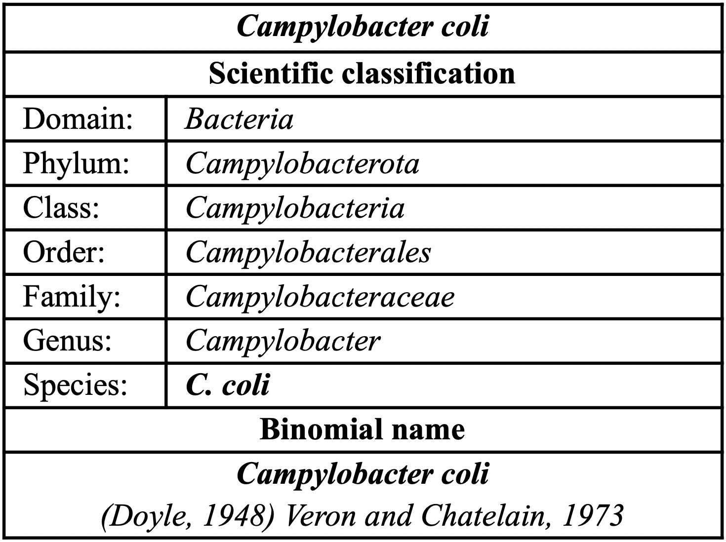
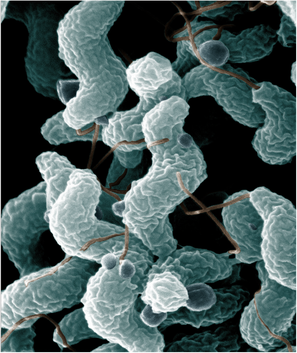
Campylobacter coli (C. coli) is a gram-negative, S-shaped bacteria within the genus Campylobacter (Prescott LM, 2005). This type of bacteria is distinguished by its microaerophilicity: with prolonged exposure to air, they acquire a coccidoid or spherical shape. Thereby, the above-mentioned organism is extremely sensitive to any changes in the external environment. Aerobic conditions, fluctuating temperature and osmotic pressure, as well as hunger, put the bacterium into a state of stress. Nonetheless, it should be noted that in the genus Campylobacter C. coli is more aerotolerant than C. jejuni, the closest specimen to the one under study (Karki et al., 2019). Some research has shown that the optimal temperature for the normal activity is considered to be 42C (Allos, B. M., 2001).
C. coli causes campylobacteriosis in humans, the most commonly reported diarrheal foodborne illness (EFSA Journal, 2018). Representatives of the genus are thought to be primarily transmitted to humans by ingestion of contaminated fresh foods such as meat and milk. There are several virulence factors that determine the ability of C. coli to cause disease. These include adhesion, invasion and bacterial motility adherence. Campylobacter secrete cytolethal distending toxin (CDT), which is an AB toxin that has DNase activity that causes DNA double-strand breaks during the G2 phase of the cell cycle. This eventually leads to apoptosis in the cells (Prescott LM, 2005).
Data on the genome and proteome of the studied bacterium were taken from the database of the National Center for Biotechnology Information (NCBI). Most of the research was done using spreadsheet functionality, the Python programming language, and the EMBOSS bioinformatics package installed on kodomo. All data was additionally verified using third-party programs, which include UGENE. This method was chosen exclusively to improve the quality and reliability of the results. Additional studies are based on the use of all the above methods.
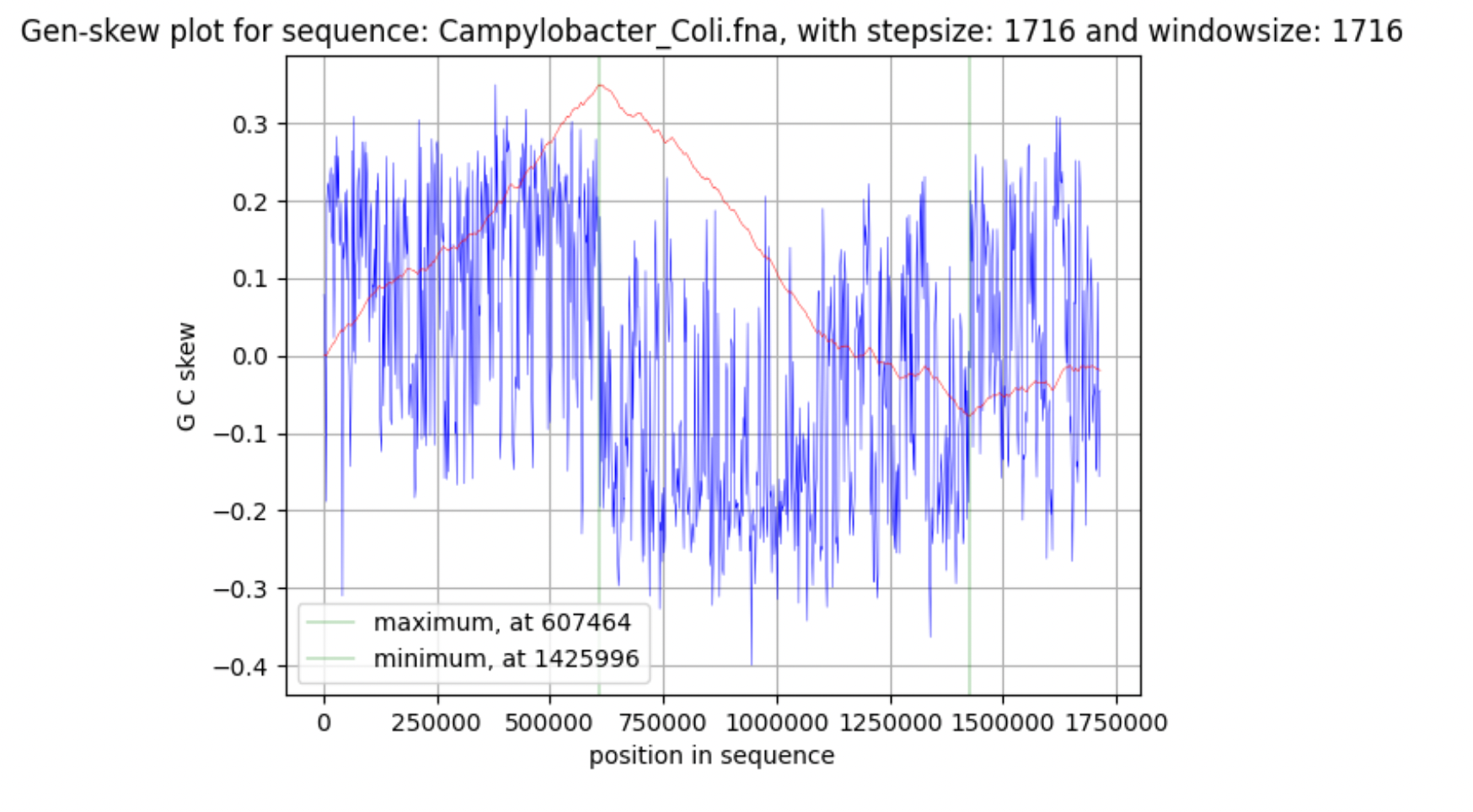
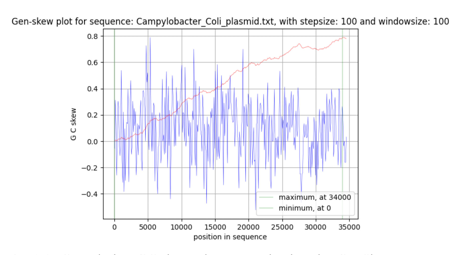
Basic data on the genome of the bacterium (nucleotide and amino acid sequences, table of features of the bacterium) were taken from the database of the National Center for Biotechnology Information (NCBI) (Supplementary materials 5,6). Further, the GenSkew program (Jennifer Lu, 2022) was used to plot the GC-skew diagram. Minimum and maximum cumulative GC skew have been analyzed using the online version of the Genskew program (Jennifer Lu, 2022). GenSkew calculates the incremental and the cumulative skew of two selectable nucleotides for a given sequence according to the formula: GC skew = (G - C) / (G + C) The GC composition of the chromosome and plasmid was analysed using the EMBOSS bioinformatics package, or rather, the geece command.
As an additional study, we conducted a reading frame and site restriction analysis. For this, the Unipro UGENE program was used. All figures were also built in the above program.
The basic sequence data was obtained from the NCBI (Supplementary materials 5, 6). Using a table of features of a bacterium (Supplementary material 1) we counted the number of genes (the count was made line by line, using a filter). To analyze the frequency of occurrence of codons encoding amino acids, we used a code written in Python (Supplementary materials 4, paragraph 1, 2). Codons were intentionally sorted alphabetically for easy interaction with the received data. For the frequency of occurrence of amino acids and individual nucleotides, the code written in the Python programming language was also used (Supplementary material 4, paragraph 3).
To analyse the proteome, a table of features of the Campylobacter coli was imported into Google Spreadsheets. For convenience, a column of so-called “pockets” was placed in the table, indented by 30 amino acids (Supplementary material 2). Then it was calculated how many proteins with a length, the value of which falls into a given “pocket”, are contained in each interval (Fig. 7). For this, the standard function COUNTIFS (Excel) was used.
As one of the additional studies, it was decided to find out how many proteins are contained in + and - DNA strands respectively. As for the previous analysis, the built-in Excel functions were used: =COUNTIF(CDS!E:E; “+”), =COUNTIF(CDS!E:E; “-”), where CDS!E:E is a reference to the “strand” column in the table of the genome of the bacterium in question (Supplementary material 1).
To find ribosomal proteins, filters were applied on two columns: “#feature” and “name”, in which the values “CDS” and “ribosomal” were searched (Supplementary material 1).
The number of hypothetical proteins was counted using the built-in Excel function: =IFERROR(VLOOKUP(“hypothetical”,B1,1)+). A table of features of the bacterium was also used (Supplementary material 1).
Using the VLOOKUP function mentioned in the previous paragraph and additional rechecking of the obtained data using built-in filters (it was applied to a table of features of a bacterium; supplementary material 1), the number of transport proteins was calculated.
With the help of filters (“RNA”) and a table of features of the observed bacterium (Supplementary material 1) we counted the number of RNA genes in the proteome.
It was found that the length of the chromosome is 1678432 bp, the plasmid - 38104 bp. Further, these data were directly involved in the study. Talking about the chromosome, the maximum value corresponds to the region ter (607464 bp), in which replication is terminated, and the minimum value corresponds to oriC (1425996 bp), in which it begins.
Using the EMBOSS bioinformatics package it was found that the proportion of guanine (G) and cytosine (C) among all
nucleotide residues of the considered chromosome is 31,41%. The GC-content of the plasmid, in turn, is 28% (Table 2.1 and Table 2.2).
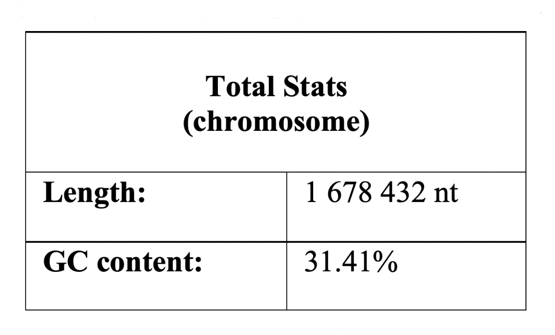
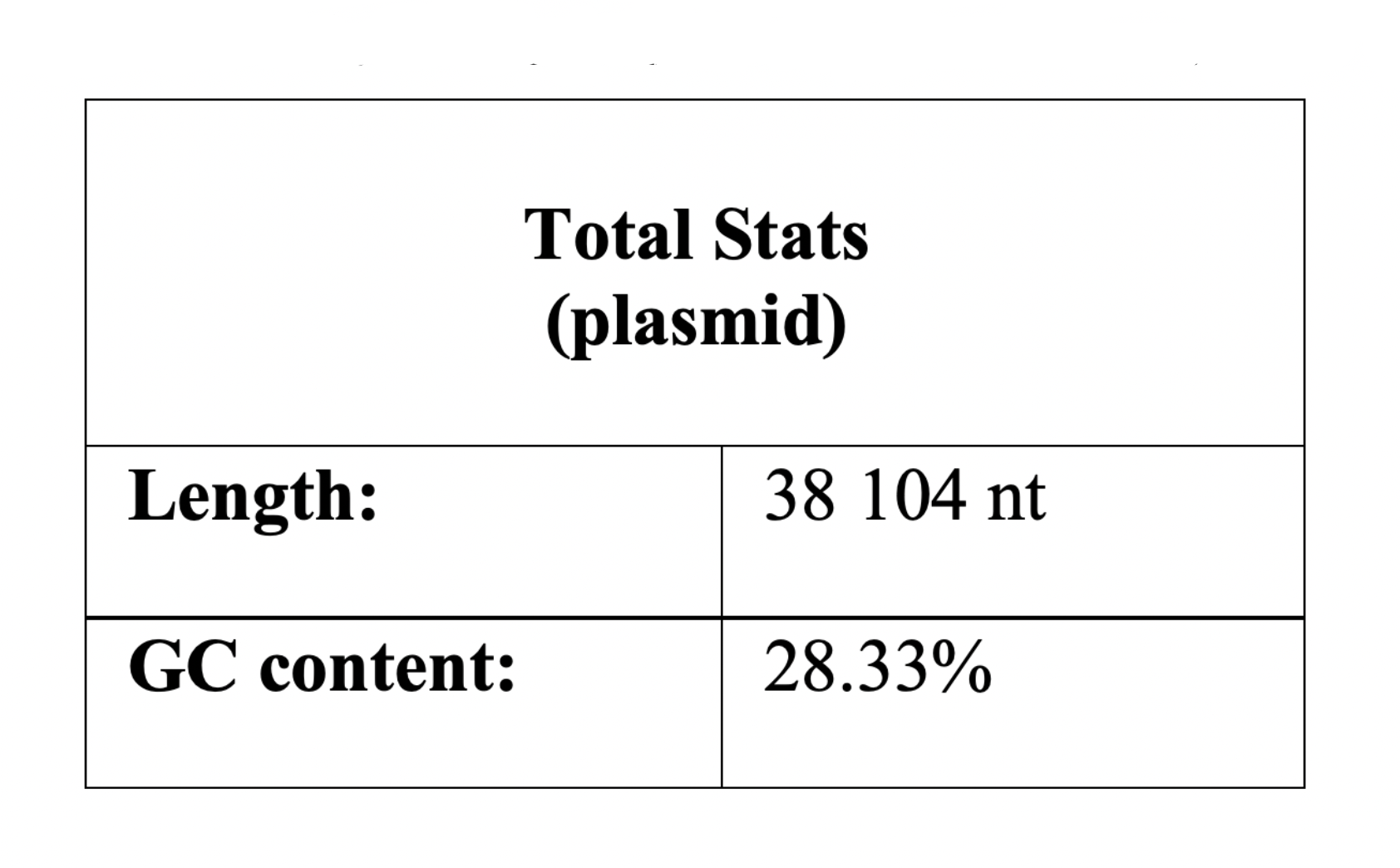
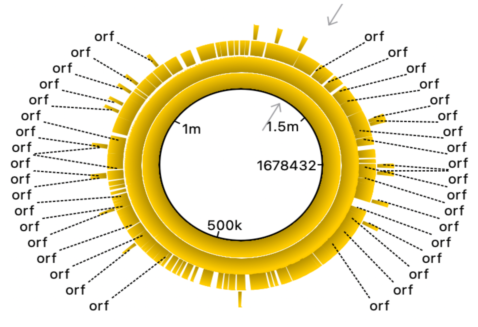
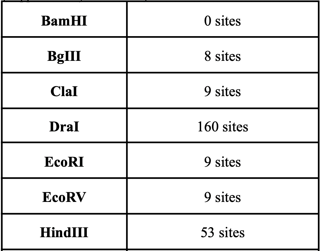
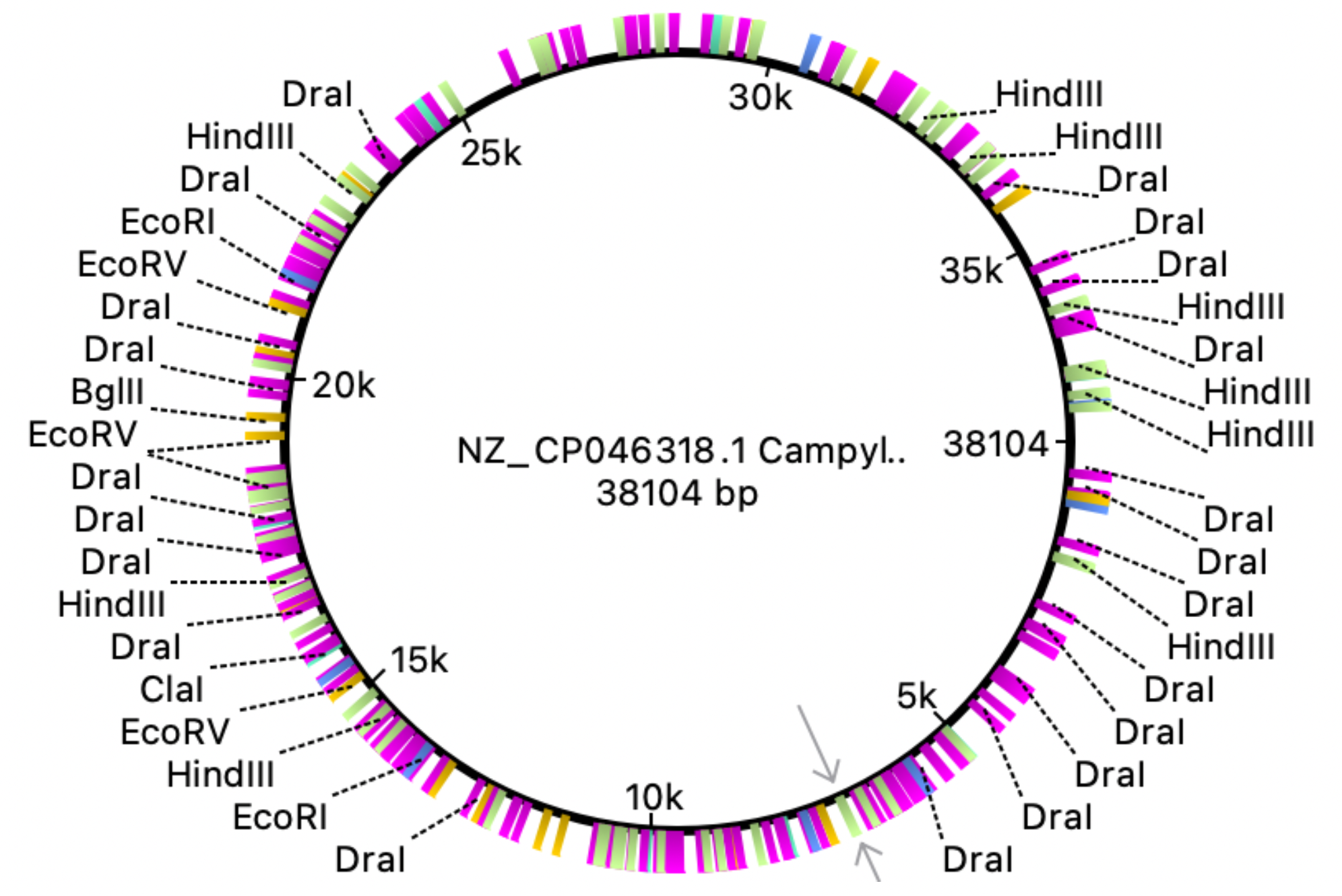
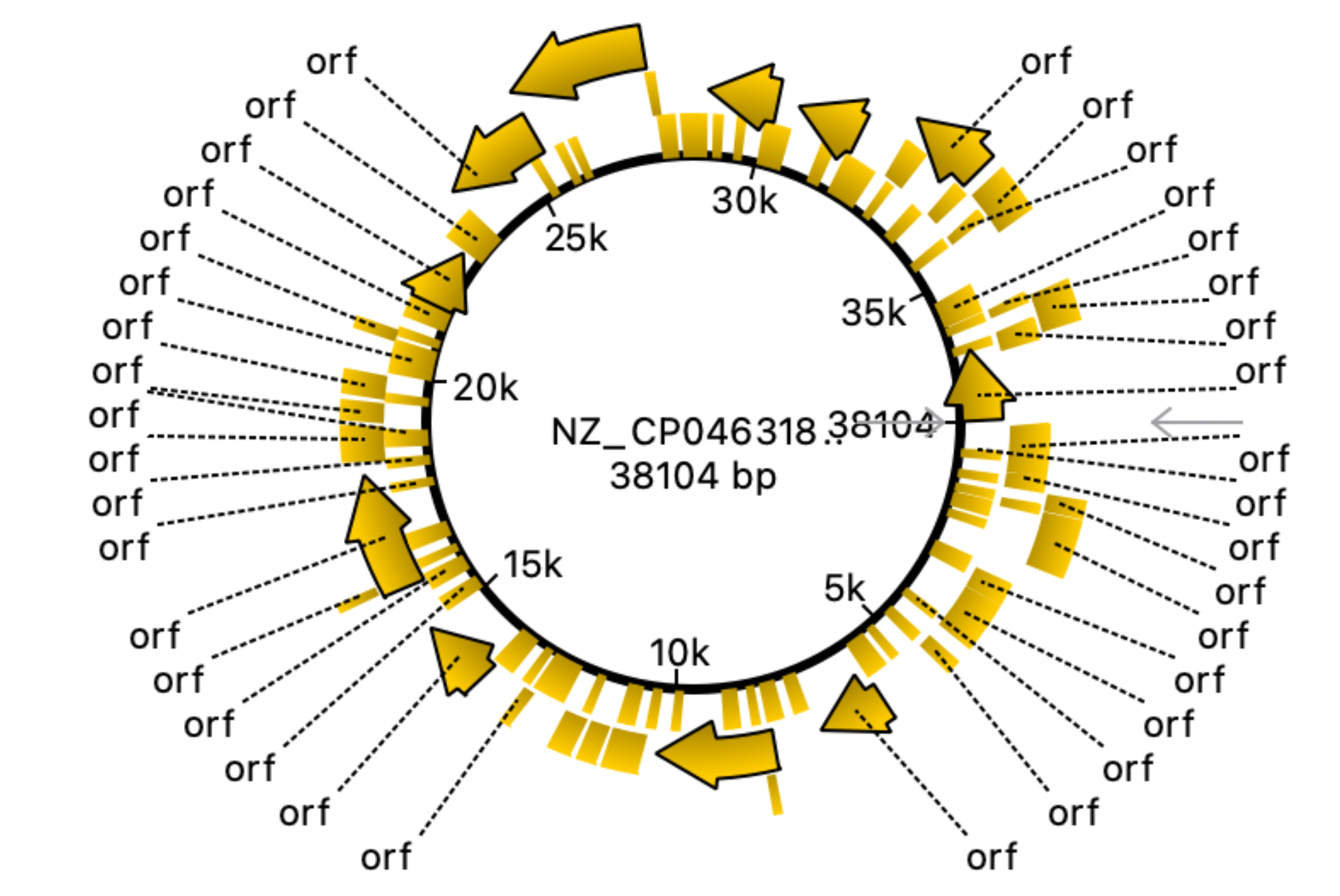
Fig. 3 and 4 clearly illustrate the approximate location of open reading frames and restriction sites, respectively. Additionally, Table 3.1 is provided showing the number of relevant restriction sites.
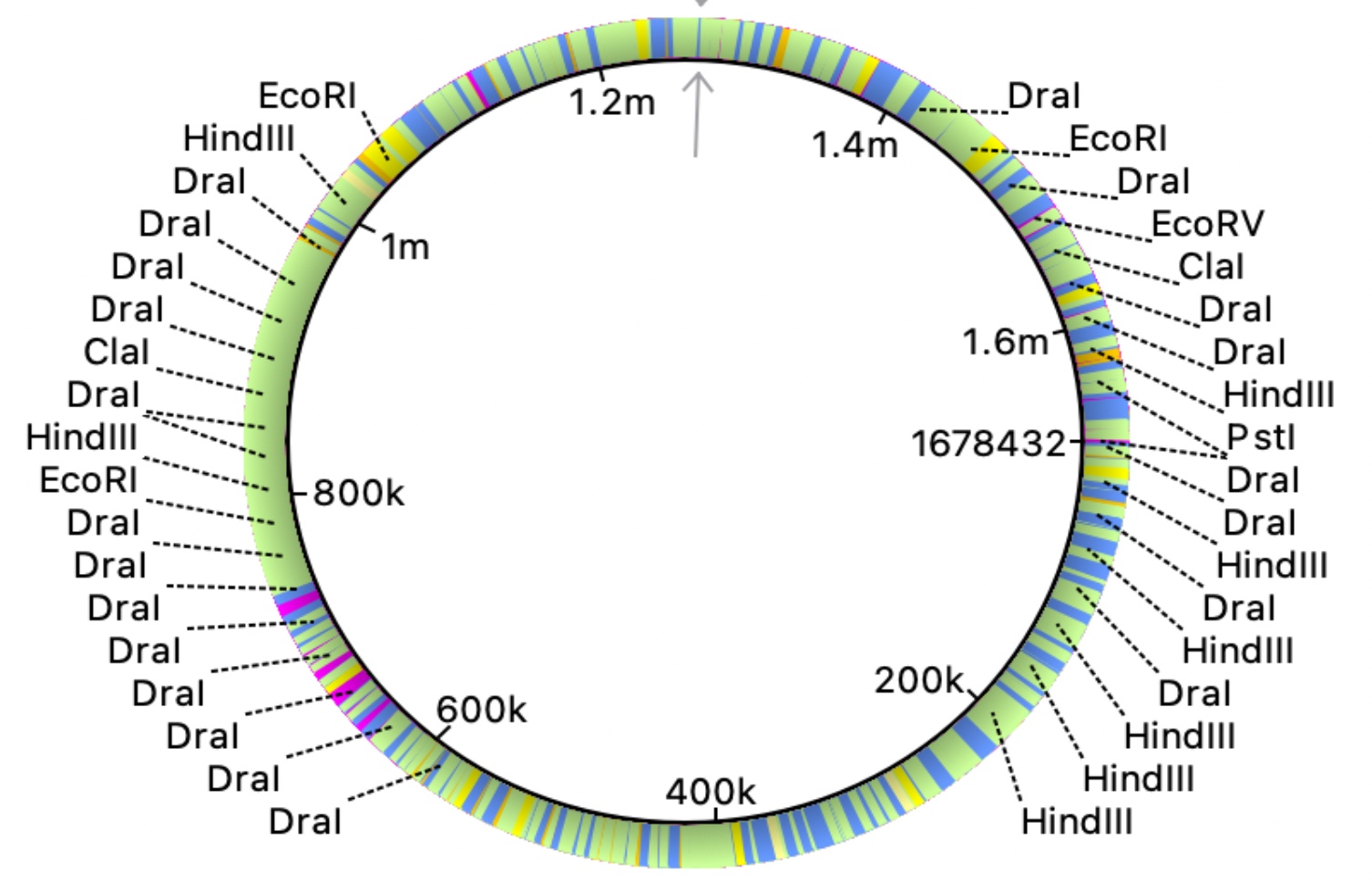
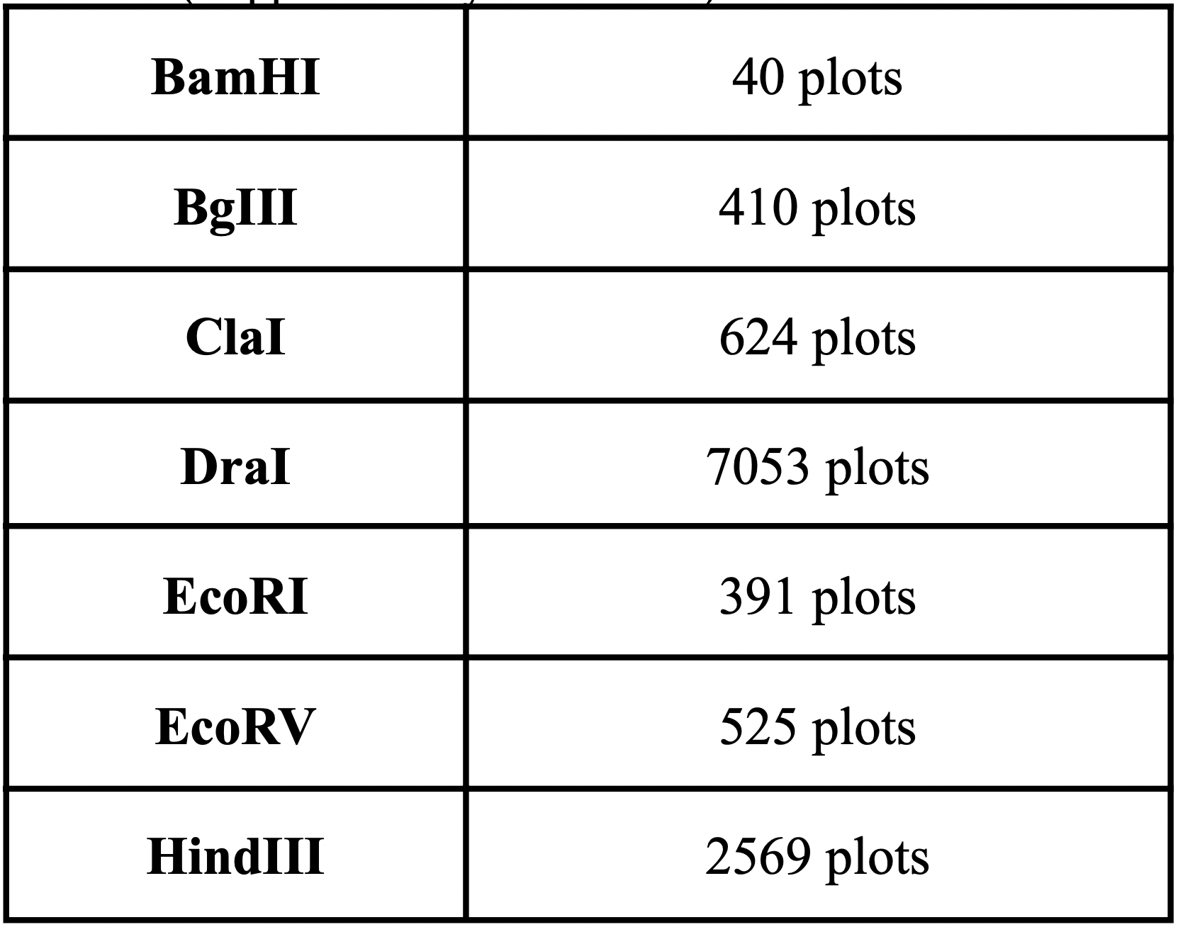
A restriction site is a sequence of approximately 6-8 base pairs (bp) of DNA that binds to a given restriction enzyme. Restriction enzymes are produced by bacteria in the course of evolution in order to destroy foreign DNA that can enter the cell and cause its transformation. Restriction sites are important for facilitating the insertion of target genes into various constructs such as plasmids. A large number of the following restriction sites were found in the genome: HindIII (2569 plots; serves as an enzyme that cleaves the palindromi sequence AAGCTT by hydrolysis), DraI (7053 plots; serves as an endonuclease for accelerated DNA (TTT^AAA) hydrolysis) (Erik K.R. Hanko, 2019).
The results are quite understandable. Bacteria have restriction sites containing large amounts of thymine (T) and adenine (A). In 2007, a study was conducted that showed that campylobacterophage DNA is practically not cleaved by enzymes whose recognition sites contain the bases cytosine (C) and guanine (G) due to an as yet unknown DNA modification (Hansen, V.M.; Rosenquist, H., 2007). In contrast, restriction endonucleases that recognize pure A/T sequences (eg, DraI) can be used to cut phage DNA and compare restriction patterns on standard agarose gels, allowing cost-effective and time-saving analysis. Open reading frames (ORFs) are defined as spans of DNA sequence between the start and stop codons. The resulting images clearly illustrate the data of the tables with the features of the genome of the bacterium observed. All the same was done for the plasmid, using the same algorithms:
The complete genome of the bacterium that is the object of study consists of a chromosome (1.678.432 bp) and a single plasmid
(38.104 bp), as mentioned above. According to the table of features of the bacterium, we found that the total number of genes
is 1778 (all kinds of genes are included).
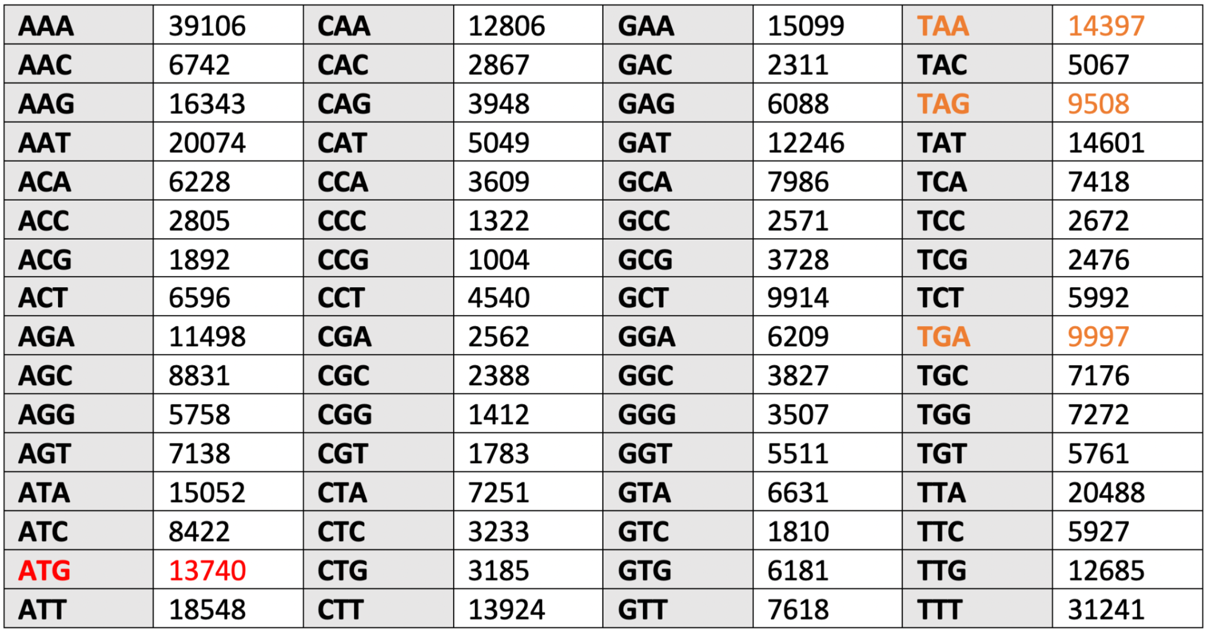
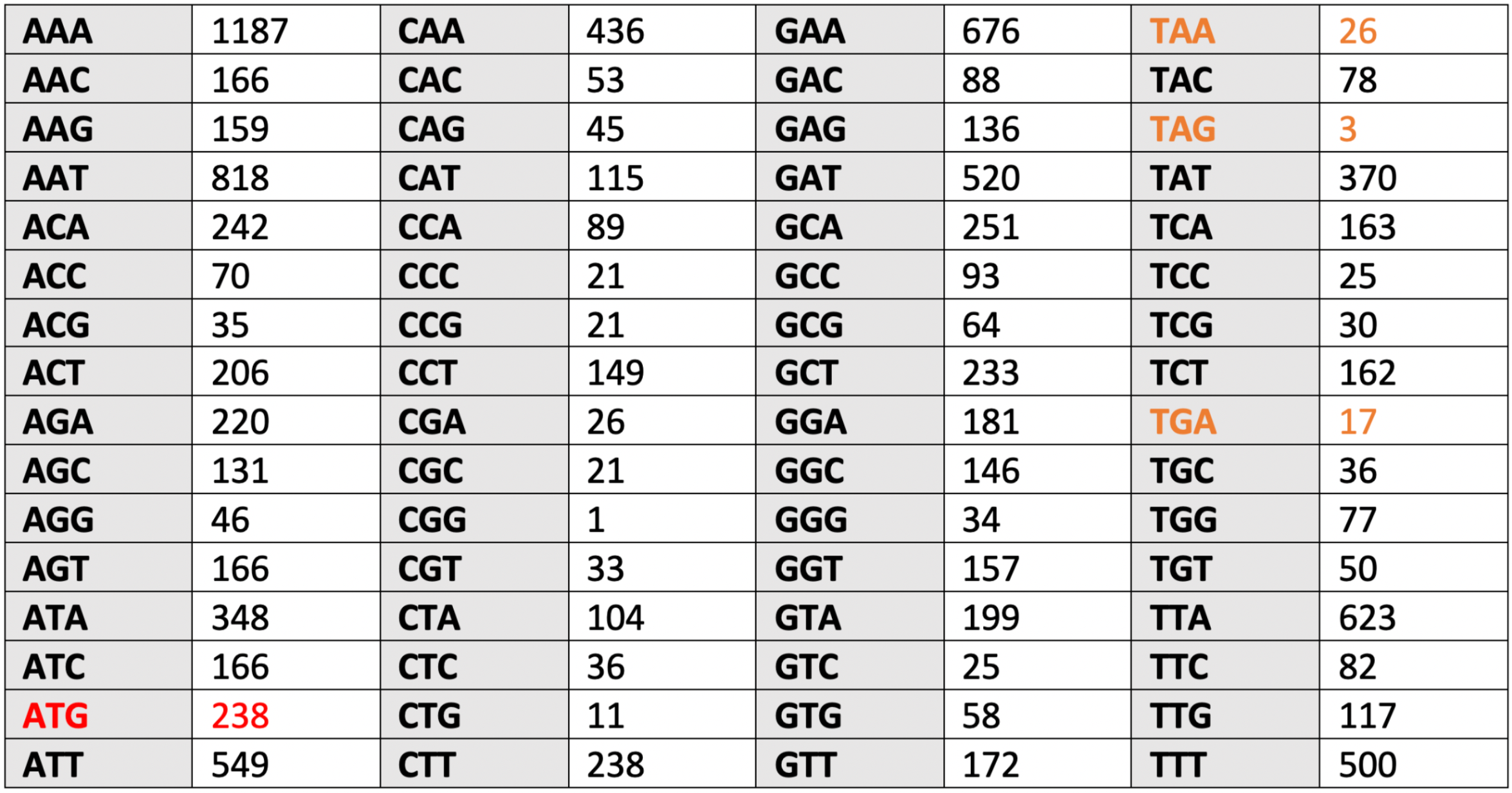
The results of counting the frequency of occurrence of codons for chromosome and plasmid are shown in Table 5.1 and Table 5.2.
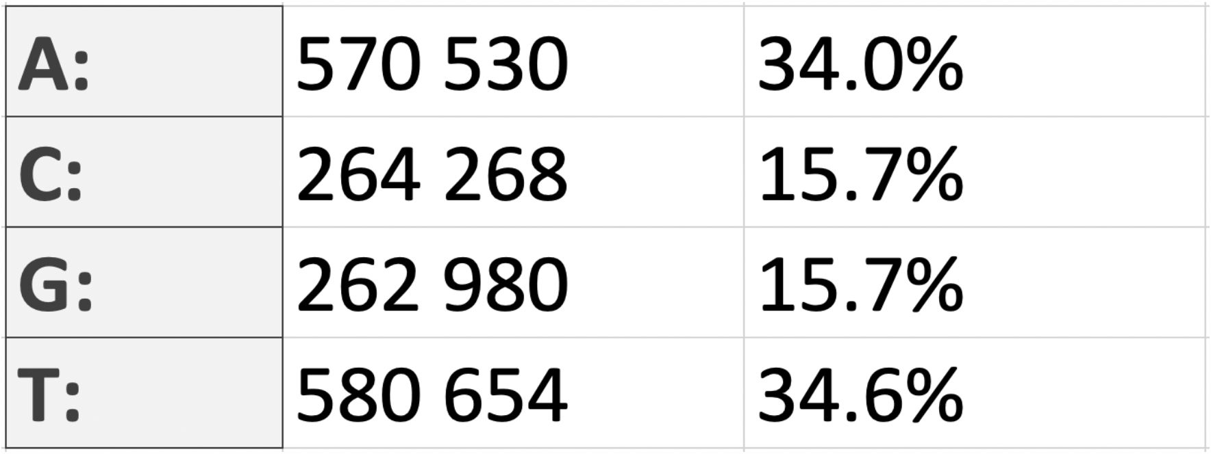
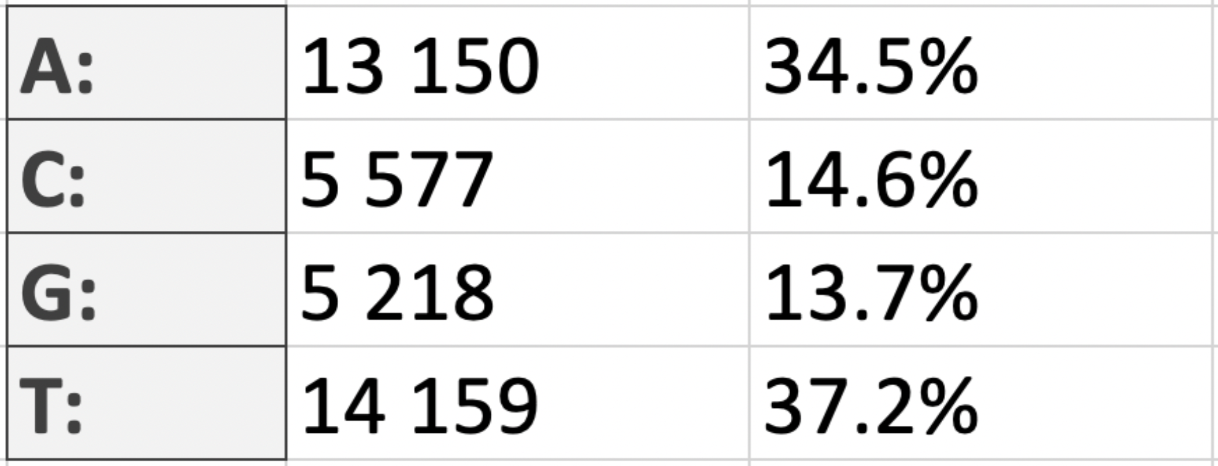
On right are tables showing the nucleotide composition of the chromosome and plasmid (Table 4.1 and Table 4.2).
The result obtained fully confirms the second Chargaff rule, which establishes the equality of the oligonucleotides that read the
same in opposite directions, taking into account the replacement of nucleotides according to the complementarity rule: the amount of
adenine (in our case, 570.530 nt) is approximately equal to the amount of thymine (580.654 nt), and guanine (262.980 nt) - to cytosine
(264.268 nt); A=T, G=C. This can be confirmed by calculations: the percentage of A from the sum of A and T is 49,5; the percentage of G
from the sum of C and G is 49,88. As we can see, the values (talking about the chromosome) are really very close to the “50/50” ratio.
Below is a graph showing the distribution of proteins by their lengths, generated using spreadsheet methods.
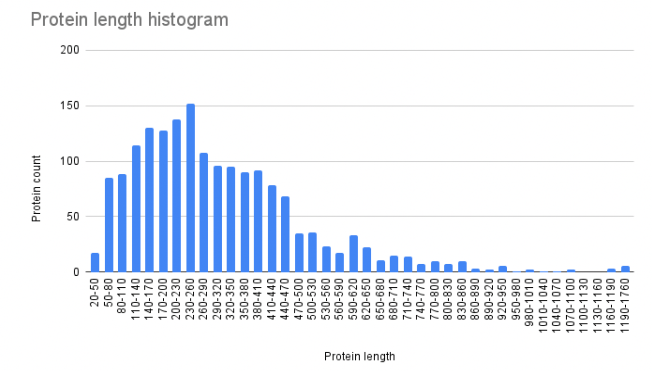
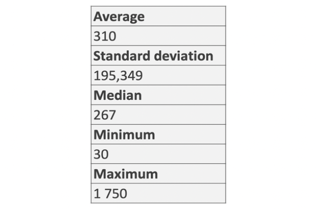
It’s worth noting that the histogram has a positive asymmetry
(there is a long right “tail”). The mean value for a distribution
with positive asymmetry is known to be larger than the median, which
is confirmed by another table indicating the main aspects of the
protein composition of the molecule (Table 7). Thus, such a
two-humped distribution of Campylobacter coli is characteristic
of many archaea.
Interestingly, the minimum length of a
protein is 30 and the maximum is 1750 amino acids.
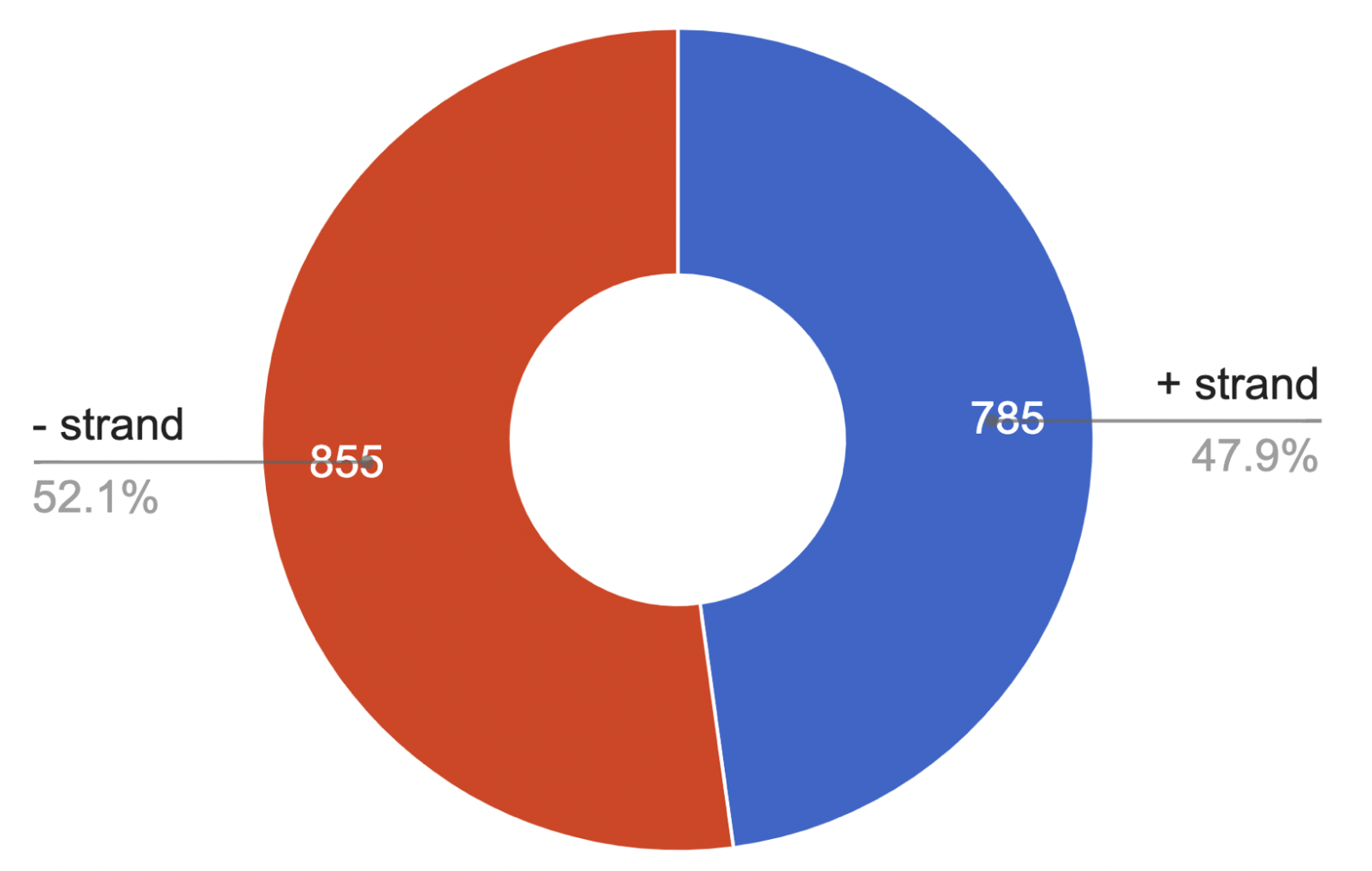
We found that there are 855 proteins on the forward strand and 785 - on the
reverse. The result is presented in Fig. 8.
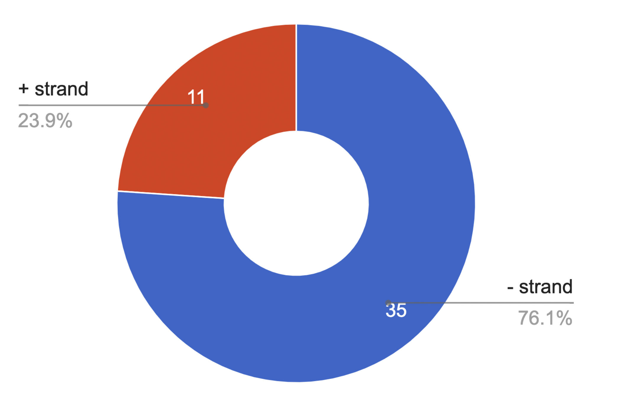
A different distribution is found in the plasmid: 11 proteins are located on the forward strand, 35 - on the reverse. The result is presented in Fig. 9.
Using the above spreadsheet methods it was found that there are 56 ribosomal proteins in the proteome.
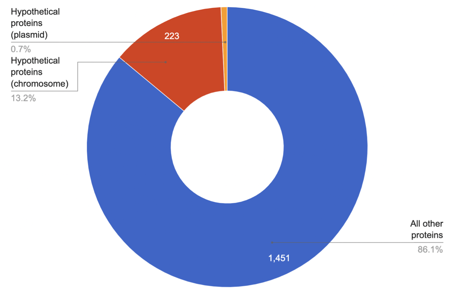
The result of the search for hypothetical proteins is shown in the diagram (Fig. 10).
As can be seen, the proteins whose existence was predicted, but for which there is no experimental
evidence that it is expressed in vivo, are 13,9% of the proteome. It may be possible to predict the
function of these proteins by searching for domain homology with different levels of confidence,
or by using homology modelling, in which a hypothetical protein must correspond to a known protein
sequence whose three-dimensional structure is known.
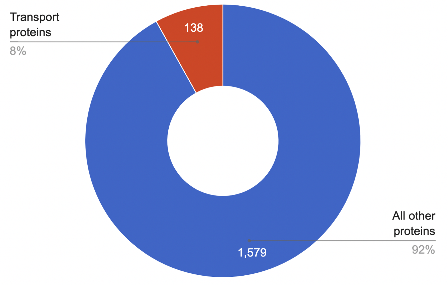
138 transport proteins of various functions were
found to be presented in the proteome. Their contribution to
the proteome is shown in the diagram (Fig. 11).
As we can see, transport proteins make up a relatively small
part of the proteome: their number correlates with the amount of
all other proteins with a coefficient of 0,087. In terms of percentage,
transport proteins occupy 4/25 of the entire proteome. The obtained data
are quite consistent with the statistical distribution.
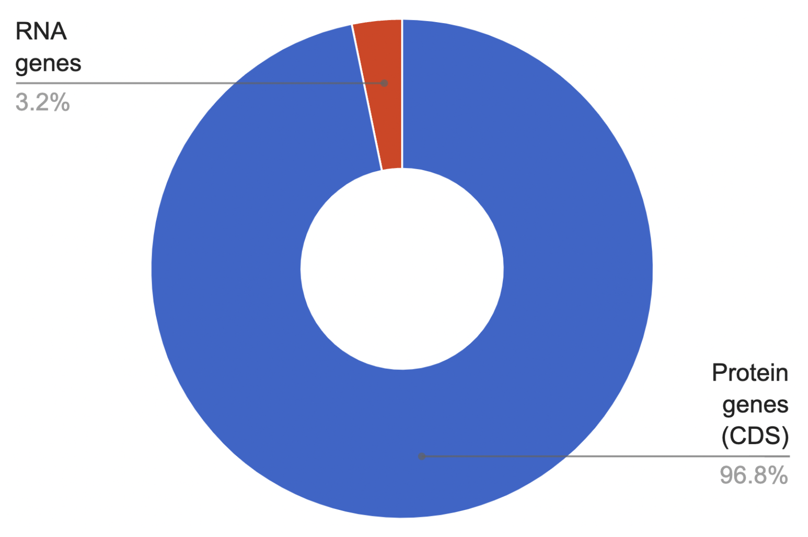
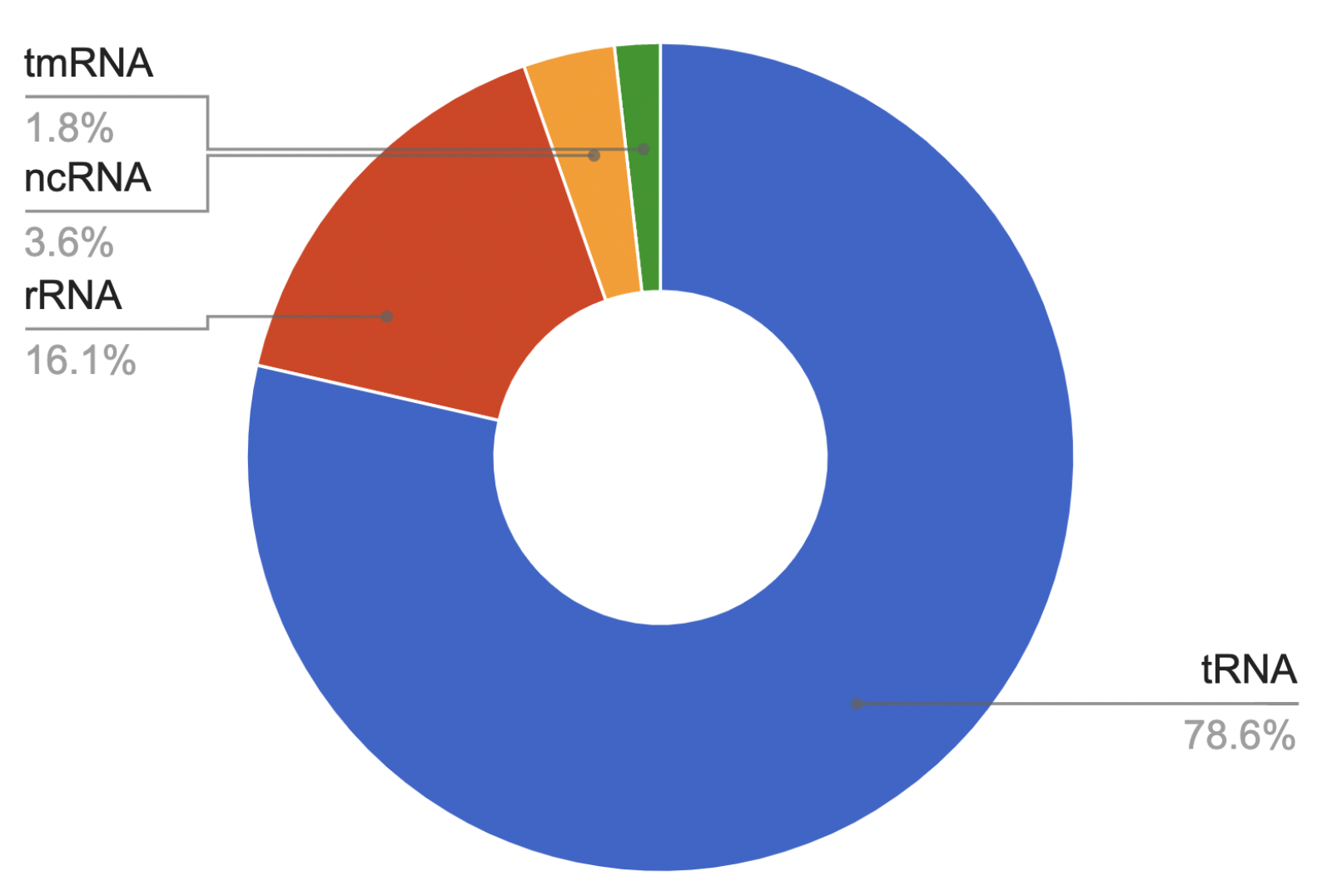
We found that the genome contains 56 RNA genes: 44 tRNAs, 9 rRNAs, 2 ncRNAs and 1 tmRNA. The pie chart (Fig. 12) clearly shows the percentage of RNA genes in the total number of genes. The second pie chart (Fig. 13) reflects the percentage of RNA genes relative to each other.
1. Allos, B. M. (2001). Campylobacter jejuni infections: Update on emerging issues and trends. Clinical Infectious Diseases, 32(8), 1201-1206.
2. Erik K.R. Hanko, Nigel P. Minton, Naglis Malys, Chapter Nine - Design, cloning and characterization of transcription factor-based inducible gene expression systems. Methods in Enzymology, Academic Press, Volume 621, 2019, pages 153-169.
3. Hansen, V.M.; Rosenquist, H.,; Baggesen, D.L.; Brown, S.; Christensen, B.B. Characterization of Campylobacter Phages Including Analysis of Host Range by Selected Campylobacter Penner Serotyopes. BMC Microbiol. 2007, 7, 90. [Google Scholar] [CrossRef] [PubMed]
4. Karki A.B., Wells H., Fakhr M.K. Retail liver juices enhance the survivability of Campylobacter jejuni and Campylobacter coli at law temperatures. Sci. Rep. 2019;9:2733. [PMC free article] [PubMed] [Google Scholar].
5. Prescott LM, Harley JP, Klein DA (2005). “Campylobacter”. Microbiology (6th ed.). pp. 430-433, 500.
6. SkewIT,
https://journals.plos.org/ploscompbiol/article?id=10.1371/jou rnal.pcbi.1008439 (06.04.2022), SkewIT: The Skew Index Test for large scale GC Skew analysis of bacterial genomes, Steven L. Salzburg. Specific link: https://genskew.csb.univie.ac.at/webskew
7. The European Union One Health 2018 Zoonoses Report, EFSA Journal.