Lin Yanbo
Faculty of Bioengineering and Bioinformatics, Lomonosov State University, Moscow, Russia
Abstract: Nowadays, we possess plenty of methods to analyze origins or affiliations of most known creatures, including bacteria, archaea. Here, we analyze the V. Halodenitrificans, which were isolated from salt salterns, in fundamental ways.
Keyword: Bacteria, Genomics, BASH, Excel, Data
Salinity, which is a common natural phenomenon of arid and semiarid regions, has already caused innumerable damages by the presence of salts and bicarbonates in soil and water to agriculture, infrastructure, environment and so on (“Types of salinity | Environment, land and water”). Besides, salt kill much types of bacteria by the brut-
al way — osmosis, meanwhile, some types of bacteria treat saline environment as their habitat, for an instance, the species Virgibacillus halodenitrificans which is a mem-
ber of genus Virgibacillus whose species have been mostly isolated from saline envir-
onments (Rosenberg et al. 2013). You probably have already had curiousness of their
halotolerant property, hence I would firstly use the fundamental analytic methods to rudimentarily learn about one of Virgibacillus - Virgibacillus halodenitrificans in several basic aspects.
— MATERIALS
At the beginning of all, we would abstract the data of Virgibacillus halodenitrif-
icans, which is named as ”GCF_001878675.1_ASM187867v1”, from ncbi.nlm.nih.gov.
— METHODS
In the analytic part, we are going to analyze ”GCF_001878675.1_ASM187867v1” in two aspects of DNA, protein, RNA, chromosome respectively.
a. DNA
In this step, the BASH program is an essential tool to digitally precisely calcul-
ate the quantity of DNA which retain in the genome with each length. Firstly we would create( mkdir ) a directory which is named ”review_VH” to save the data of ”GCF_0018-
78675.1_ASM187867v1”. Then we could create and write a shell script which is named “count_dna.sh” to process calculation by list and save the calculated data in a vi-
sual file(Fig.1).In this script, we use ”cut”( pick the columns which we need),”sed”( cut the heading ),”grep”( select DNA among them ) and ”wc”( calculate the quantity of DNA ) respectively, at the end, it is to keep the data in a visual file data_vh.txt.
Fig.1 The executing codes in the shell script
Hence, using this method lets us visually recognize the 89 DNA and their each
length. Also, from another data file GCF_001878675.1_ASM187867v1_assembly_stats.txt, we could know that the percentage of retained GC-pairs in the genome is 37.5%, also the total length is 3917759, therefore we could get the quantity of retained GC-pairs is about 1469160 by the general arithmetic.
b. Protein
Here we start toward this step - to learn about the proteome of Virgibacillus halo-
denitrificans. It is to compile the data of that in several aspects which are the ap-
proximate comparison of lengths of proteins(below as ACLP) , the comparison between the quantity of the translated protein genes in straight and complementary chains (B-
elow as CTSC), the determination of the quantity of ribosomal proteins (Below as DQ-
RP),the determination of the quantity of the hypothetical protein which didn’t be de-
termined(Below as DQHP) and the determination of the quantity of the transport proteins separately(Below as DQTP). We would execute them step by step.
— ACLP
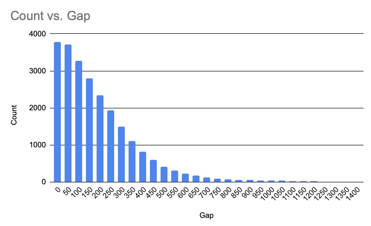
Here we would use another tool to make an approximate statistics — Excel. Firstly it is to import the data file into a new sheet, then copy the ”chromosome”,”star-
t”,”end”, ”strand”, ”product_accession”, ” name” and ” product length” columns to an additional sheet which is named as ”CDS”, after all of them, we make another sheet for making a histogram of the comparison, we would set comparative gaps each which is 50, then by the gas we could the formula ”fx=COUNTIFS(CDS!H:H,">="&A(ɑ))” to get the quantity of proteins which are longer than the supremum of the gap, we could make a histogram easily by the data(Fig.2).
Fig.2 The histogram of ACLP
— CTSC
Here we would still use the COUNTIFS formula to calculate the quantities of the ”+” and ”-” strands of the coding proteins, but the difference from ACLP is that we would use the filter tool. Firstly, it is to make a filter ”protein_coding” in the class column in the imported sheet to pick the coding proteins up, then copy the filtered ”strand” column to a new sheet which is named ”cod-
ing protein strand” as the A column, after that, put the formulas ”fx= COUNTIFS(A:A,"+")” and ”fx= COUNTIFS(A:A,"-")” in two cells respectively, then we would get the digital result that in the coding proteins are 2015 ”+” strands and 1762 ”-” strands.
— DQRP and DQHP
Mostly same as CTSC, the formulas for the ribosomal proteins and the hypothetical proteins are ”fx =COUNTIFS(A:A,"*ribosomal protein*")” and ” fx = =COUNTIFS(A:A,"*hypothetical protei-
n*")”, by them, we could know that there are 58 ribosomal proteins and 514 hypothetical proteins.
– DQTP
Still mostly same as CTSC, the formulas for the transporter proteins is ” fx = =(COUNTIFS(A:A,
"*transporter*protein*"))”, then we could know that there are 106 transporter proteins in that, also put the formula ”fx = COUNTIFS(A:A,"*protein*")” to get the quantity of proteins in that, then we could calculate out the percentage of the transporter proteins from all proteins — 5.38%.
c. RNA
We have already used the data file to get parts of the needed data via excel. Here, we could easily compile some statistics by the same method.Here we could know that there are 207 RNA, 24 ribosomal RNA and 115 tRNA.
d. Chromosome
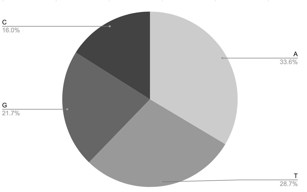
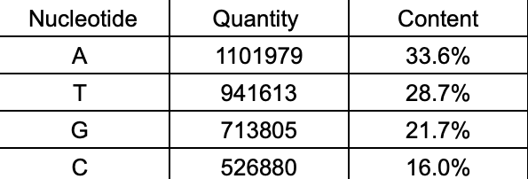
In this step, we would use BASH programs to calculate each content of A, T, G, C nucleotides in the DNA. On the same method, it is to use BASH programs to get the quantities, here I make a shell script(Fig.3) to execute the calculation, then get the result file which record that there are 11-
01979 A nucleotides, 941613 T nucleotides, 713805 G nucleotides and 526880 C nucleotides. Meanwhi-
le, we could use the same method as the ” ACLP ” step to visually and digitally compare their con-
tents by pie chart (Fig.4-1,4-2).

Fig.3 The codes of the shell script.
Fig.4-1 The pie chart which includes the cont- Fig.4-2 The table of data of each nucleotide.
ent of each nucleotide.
To learn about bacteria and archaea in the basic aspect including DNA, protein, RNA, chromosome, we could grab their genetic information from ncbi.nlm.nih.gov(NATIO-
NAL CENTRE FOR BIOTECHNOLOGY INFORMATION) and analyze that by usage of the elementary methods, which are BASH programs and Excel, visually and digitally.
GCF_000195275.1_ASM19527v1_feature_table.txt
GCF_001878675.1_ASM187867v1_assembly_stats.txt
GCF_001878675.1_ASM187867v1_cds_from_genomic.fna
Rosenberg, Eugene, et al., editors. The Prokaryotes: Prokaryotic Biology and Symbiotic
Associations. Springer Berlin Heidelberg, 2013.
“Types of salinity | Environment, land and water.” Queensland Government,8 October 2013, https://www.qld.gov.au/environment/land/management/soil/salinity/types. Accessed 29 Ja-
nuary 2023.