Вычисление атомных орбиталей водорода
В этом практикуме необходимо, опираясь на уравнение, построить электронную плотность в одноэлектронном атоме и сравнить с выдачей известных программ.
Импортируем модули и функцию Андрея Демкива.
import numpy
import scipy.special
import scipy.misc
import npy2cube
Задаем волновую функцию:
def w(n,l,m,d):

    x,y,z = numpy.mgrid[-d:d:30j,-d:d:30j,-d:d:30j]

    r = lambda x,y,z: numpy.sqrt(x**2+y**2+z**2)
    theta = lambda x,y,z: numpy.arccos(z/r(x,y,z))
    phi = lambda x,y,z: numpy.arctan(y/x)

    a0 = 1.

    R = lambda r,n,l: (2*r/n/a0)**l * numpy.exp(-r/n/a0) * scipy.special.genlaguerre(n-l-1,2*l+1)(2*r/n/a0)
    WF = lambda r,theta,phi,n,l,m: R(r,n,l) * scipy.special.sph_harm(m,l,phi,theta)
    absWF = lambda r,theta,phi,n,l,m: numpy.absolute(WF(r,theta,phi,n,l,m))**2

    return WF(r(x,y,z),theta(x,y,z),phi(x,y,z),n,l,m)
# определим шаг grid при заданном диапозоне от -d до d
d = 50
step = float(d/30)
# зададим цикл по перебору квантовых чисел

for n in range(0,4):
    for l in range(0,n):
        for m in range(0,l+1,1):
            grid = w(n, l, m, d)
            name='grid3/%s-%s-%s' % (n,l,m)
            # для сохранения нужно задать координаты старта grid и шаг по каждому направлению
            npy2cube.npy2cube(grid,(-d, -d, -d),(step, step, step),name+'.cube')
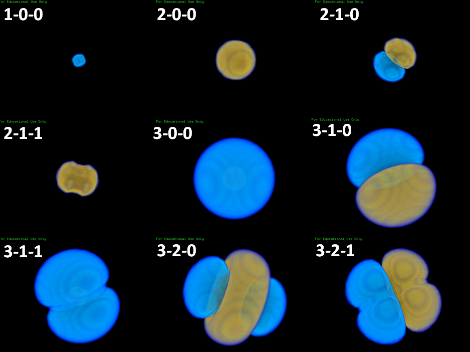
Получили такие изображения орбиталей. Если уменьшить параметр d до 50, становится видна и 1s орбиталь.
Теперь попробуем рассчитать орбитали в программе ORCA. Создаем файл h3.inp для orca и запускаем ее:
%%bash
export PATH=${PATH}:/tmp
orca h3.inp
*****************
* O R C A *
*****************
--- An Ab Initio, DFT and Semiempirical electronic structure package ---
#######################################################
# -***- #
# Department of molecular theory and spectroscopy #
# Directorship: Frank Neese #
# Max Planck Institute for Chemical Energy Conversion #
# D-45470 Muelheim/Ruhr #
# Germany #
# #
# All rights reserved #
# -***- #
#######################################################
Program Version 3.0.0 - RELEASE -
With contributions from (in alphabetic order):
Ute Becker : Parallelization
Dmytro Bykov : SCF Hessian
Dmitry Ganyushin : Spin-Orbit,Spin-Spin,Magnetic field MRCI
Andreas Hansen : Spin unrestricted coupled pair/coupled cluster methods
Dimitrios Liakos : Extrapolation schemes; parallel MDCI
Robert Izsak : Overlap fitted RIJCOSX, COSX-SCS-MP3
Christian Kollmar : KDIIS, OOCD, Brueckner-CCSD(T), CCSD density
Simone Kossmann : Meta GGA functionals, TD-DFT gradient, OOMP2, MP2 Hessian
Taras Petrenko : DFT Hessian,TD-DFT gradient, ASA and ECA modules, normal mode analysis, Resonance Raman, ABS, FL, XAS/XES, NRVS
Christoph Reimann : Effective Core Potentials
Michael Roemelt : Restricted open shell CIS
Christoph Riplinger : Improved optimizer, TS searches, QM/MM, DLPNO-CCSD
Barbara Sandhoefer : DKH picture change effects
Igor Schapiro : Molecular dynamics
Kantharuban Sivalingam : CASSCF convergence, NEVPT2
Boris Wezisla : Elementary symmetry handling
Frank Wennmohs : Technical directorship
We gratefully acknowledge several colleagues who have allowed us to
interface, adapt or use parts of their codes:
Stefan Grimme, W. Hujo, H. Kruse, T. Risthaus : VdW corrections, initial TS optimization,
DFT functionals, gCP
Ed Valeev : LibInt (2-el integral package), F12 methods
Garnet Chan, S. Sharma, R. Olivares : DMRG
Ulf Ekstrom : XCFun DFT Library
Mihaly Kallay : mrcc (arbitrary order and MRCC methods)
Andreas Klamt, Michael Diedenhofen : otool_cosmo (COSMO solvation model)
Frank Weinhold : gennbo (NPA and NBO analysis)
Your calculation uses the libint2 library for the computation of 2-el integrals
For citations please refer to: http://libint.valeyev.net
This ORCA versions uses:
CBLAS interface : Fast vector & matrix operations
LAPACKE interface : Fast linear algebra routines
SCALAPACK package : Parallel linear algebra routines
Your calculation utilizes the basis: Ahlrichs-VDZ
Cite in your paper:
H - Kr: A. Schaefer, H. Horn and R. Ahlrichs, J. Chem. Phys. 97, 2571 (1992).
Your calculation utilizes pol. fcns from basis: Ahlrichs polarization
Cite in your paper:
H - Kr: R. Ahlrichs and coworkers, unpublished
================================================================================
WARNINGS
Please study these warnings very carefully!
================================================================================
Now building the actual basis set
INFO : the flag for use of LIBINT has been found!
================================================================================
INPUT FILE
================================================================================
NAME = h3.inp
| 1> ! UHF SVP XYZFile
| 2> %plots Format Cube
| 3> MO("H-0.cube",0,0);
| 4> MO("H-1.cube",1,0);
| 5> MO("H-2.cube",2,0);
| 6> MO("H-3.cube",3,0);
| 7> MO("H-4.cube",4,0);
| 8> MO("H-5.cube",5,0);
| 9> MO("H-6.cube",6,0);
| 10> MO("H-7.cube",7,0);
| 11> MO("H-8.cube",8,0);
| 12> MO("H-9.cube",9,0);
| 13>
| 14> end
| 15> * xyz 0 4
| 16> H 0 0 0
| 17> ** ****END OF INPUT****
================================================================================
****************************
* Single Point Calculation *
****************************
---------------------------------
CARTESIAN COORDINATES (ANGSTROEM)
---------------------------------
H 0.000000 0.000000 0.000000
----------------------------
CARTESIAN COORDINATES (A.U.)
----------------------------
NO LB ZA FRAG MASS X Y Z
0 H 1.0000 0 1.008 0.000000000000000 0.000000000000000 0.000000000000000
--------------------------------
INTERNAL COORDINATES (ANGSTROEM)
--------------------------------
H 0 0 0 0.000000 0.000 0.000
---------------------------
INTERNAL COORDINATES (A.U.)
---------------------------
H 0 0 0 0.000000 0.000 0.000
---------------------
BASIS SET INFORMATION
---------------------
There are 1 groups of distinct atoms
Group 1 Type H : 4s1p contracted to 2s1p pattern {31/1}
Atom 0H basis set group => 1
Checking for AutoStart:
The File: h3.gbw exists
Trying to determine its content:
... Fine, the file contains calculation information
... Fine, the calculation information was read
... Fine, the file contains a basis set
... Fine, the basis set was read
... Fine, the file contains a geometry
... Fine, the geometry was read
... Fine, the file contains a set of orbitals
... Fine, the orbitals can be read
=> possible old guess file was deleted
=> GBW file was renamed to GES file
=> GES file is set as startup file
=> Guess is set to MORead
... now leaving AutoStart
------------------------------------------------------------------------------
ORCA GTO INTEGRAL CALCULATION
------------------------------------------------------------------------------
BASIS SET STATISTICS AND STARTUP INFO
# of primitive gaussian shells ... 5
# of primitive gaussian functions ... 7
# of contracted shell ... 3
# of contracted basis functions ... 5
Highest angular momentum ... 1
Maximum contraction depth ... 3
Integral package used ... LIBINT
Integral threshhold Thresh ... 1.000e-10
Primitive cut-off TCut ... 1.000e-11
INTEGRAL EVALUATION
One electron integrals ... done
Pre-screening matrix ... done
Shell pair data ... done ( 0.000 sec)
-------------------------------------------------------------------------------
ORCA SCF
-------------------------------------------------------------------------------
------------
SCF SETTINGS
------------
Hamiltonian:
Ab initio Hamiltonian Method .... Hartree-Fock(GTOs)
General Settings:
Integral files IntName .... h3
Hartree-Fock type HFTyp .... UHF
Total Charge Charge .... 0
Multiplicity Mult .... 4
Number of Electrons NEL .... 1
Basis Dimension Dim .... 5
Nuclear Repulsion ENuc .... 0.0000000000 Eh
Convergence Acceleration:
DIIS CNVDIIS .... on
Start iteration DIISMaxIt .... 12
Startup error DIISStart .... 0.200000
# of expansion vecs DIISMaxEq .... 5
Bias factor DIISBfac .... 1.050
Max. coefficient DIISMaxC .... 10.000
Newton-Raphson CNVNR .... off
SOSCF CNVSOSCF .... off
Level Shifting CNVShift .... on
Level shift para. LevelShift .... 0.2500
Turn off err/grad. ShiftErr .... 0.0010
Zerner damping CNVZerner .... off
Static damping CNVDamp .... on
Fraction old density DampFac .... 0.7000
Max. Damping (<1) DampMax .... 0.9800
Min. Damping (>=0) DampMin .... 0.0000
Turn off err/grad. DampErr .... 0.1000
Fernandez-Rico CNVRico .... off
SCF Procedure:
Maximum # iterations MaxIter .... 125
SCF integral mode SCFMode .... Direct
Integral package .... LIBINT
Reset frequeny DirectResetFreq .... 20
Integral Threshold Thresh .... 1.000e-10 Eh
Primitive CutOff TCut .... 1.000e-11 Eh
Convergence Tolerance:
Convergence Check Mode ConvCheckMode .... Total+1el-Energy
Energy Change TolE .... 1.000e-06 Eh
1-El. energy change .... 1.000e-03 Eh
DIIS Error TolErr .... 1.000e-06
Diagonalization of the overlap matrix:
Smallest eigenvalue ... 3.152e-01
Time for diagonalization ... 0.000 sec
Threshold for overlap eigenvalues ... 1.000e-08
Number of eigenvalues below threshold ... 0
Time for construction of square roots ... 0.000 sec
Total time needed ... 0.001 sec
---------------------
INITIAL GUESS: MOREAD
---------------------
Guess MOs are being read from file: h3.ges
Input Geometry matches current geometry (good)
Input basis set matches current basis set (good)
MOs were renormalized
MOs were reorthogonalized (Cholesky)
------------------
INITIAL GUESS DONE ( 0.0 sec)
------------------
--------------
SCF ITERATIONS
--------------
ITER Energy Delta-E Max-DP RMS-DP [F,P] Damp
*** Starting incremental Fock matrix formation ***
0 0.0728625057 0.000000000000 0.00000000 0.00000000 0.0000000 0.7000
**** Energy Check signals convergence ****
*****************************************************
* SUCCESS *
* SCF CONVERGED AFTER 1 CYCLES *
*****************************************************
----------------
TOTAL SCF ENERGY
----------------
Total Energy : 0.07286251 Eh 1.98269 eV
Components:
Nuclear Repulsion : 0.00000000 Eh 0.00000 eV
Electronic Energy : 0.07286251 Eh 1.98269 eV
One Electron Energy: -0.31757803 Eh -8.64174 eV
Two Electron Energy: 0.39044053 Eh 10.62443 eV
Virial components:
Potential Energy : -1.57795800 Eh -42.93842 eV
Kinetic Energy : 1.65082051 Eh 44.92111 eV
Virial Ratio : 0.95586285
---------------
SCF CONVERGENCE
---------------
Last Energy change ... 0.0000e+00 Tolerance : 1.0000e-06
Last MAX-Density change ... 6.6613e-16 Tolerance : 1.0000e-05
Last RMS-Density change ... 1.0816e-16 Tolerance : 1.0000e-06
Last DIIS Error ... 5.3037e-16 Tolerance : 1.0000e-06
**** THE GBW FILE WAS UPDATED (h3.gbw) ****
**** DENSITY FILE WAS UPDATED (h3.scfp.tmp) ****
**** ENERGY FILE WAS UPDATED (h3.en.tmp) ****
----------------------
UHF SPIN CONTAMINATION
----------------------
Expectation value of <S**2> : 2.000000
Ideal value S*(S+1) for S=1.0 : 2.000000
Deviation : 0.000000
----------------
ORBITAL ENERGIES
----------------
SPIN UP ORBITALS
NO OCC E(Eh) E(eV)
0 1.0000 -0.108838 -2.9616
1 1.0000 0.572141 15.5687
2 0.0000 2.100372 57.1540
3 0.0000 2.100372 57.1540
4 0.0000 2.100372 57.1540
SPIN DOWN ORBITALS
NO OCC E(Eh) E(eV)
0 0.0000 0.487405 13.2630
1 0.0000 1.318415 35.8759
2 0.0000 2.270122 61.7732
3 0.0000 2.270122 61.7732
4 0.0000 2.270122 61.7732
********************************
* MULLIKEN POPULATION ANALYSIS *
********************************
**** WARNING: MULLIKEN FINDS 2.0000000 ELECTRONS INSTEAD OF 1 ****
--------------------------------------------
MULLIKEN ATOMIC CHARGES AND SPIN POPULATIONS
--------------------------------------------
0 H : -1.000000 2.000000
Sum of atomic charges : -1.0000000
Sum of atomic spin populations: 2.0000000
-----------------------------------------------------
MULLIKEN REDUCED ORBITAL CHARGES AND SPIN POPULATIONS
-----------------------------------------------------
CHARGE
0 H s : 2.000000 s : 2.000000
pz : 0.000000 p : 0.000000
px : 0.000000
py : 0.000000
SPIN
0 H s : 2.000000 s : 2.000000
pz : 0.000000 p : 0.000000
px : 0.000000
py : 0.000000
*******************************
* LOEWDIN POPULATION ANALYSIS *
*******************************
**** WARNING: LOEWDIN FINDS 2.0000000 ELECTRONS INSTEAD OF 1 ****
-------------------------------------------
LOEWDIN ATOMIC CHARGES AND SPIN POPULATIONS
-------------------------------------------
0 H : -1.000000 2.000000
----------------------------------------------------
LOEWDIN REDUCED ORBITAL CHARGES AND SPIN POPULATIONS
----------------------------------------------------
CHARGE
0 H s : 2.000000 s : 2.000000
pz : 0.000000 p : 0.000000
px : 0.000000
py : 0.000000
SPIN
0 H s : 2.000000 s : 2.000000
pz : 0.000000 p : 0.000000
px : 0.000000
py : 0.000000
*****************************
* MAYER POPULATION ANALYSIS *
*****************************
NA - Mulliken gross atomic population
ZA - Total nuclear charge
QA - Mulliken gross atomic charge
VA - Mayer's total valence
BVA - Mayer's bonded valence
FA - Mayer's free valence
ATOM NA ZA QA VA BVA FA
0 H 2.0000 1.0000 -1.0000 2.0000 0.0000 2.0000
Mayer bond orders larger than 0.1
-----------------------------------------------
ATOM BASIS FOR ELEMENT H
-----------------------------------------------
NSH[1] = 3;
res=GAUSS_InitGTOSTO(BG,BS,1,NSH[1]);
// Basis function for L=s
(*BG)[ 1][ 0].l = ((*BS)[ 1][ 0].l=0);
(*BG)[ 1][ 0].ng = 4;
(*BG)[ 1][ 0].a[ 0]= 13.01070100; (*BG)[ 1][ 0].d[ 0]= 0.096096678877;
(*BG)[ 1][ 0].a[ 1]= 1.96225720; (*BG)[ 1][ 0].d[ 1]= 0.163022191701;
(*BG)[ 1][ 0].a[ 2]= 0.44453796; (*BG)[ 1][ 0].d[ 2]= 0.185592186247;
(*BG)[ 1][ 0].a[ 3]= 0.12194962; (*BG)[ 1][ 0].d[ 3]= 0.073701452542;
// Basis function for L=s
(*BG)[ 1][ 1].l = ((*BS)[ 1][ 1].l=0);
(*BG)[ 1][ 1].ng = 4;
(*BG)[ 1][ 1].a[ 0]= 13.01070100; (*BG)[ 1][ 1].d[ 0]= 0.202726593388;
(*BG)[ 1][ 1].a[ 1]= 1.96225720; (*BG)[ 1][ 1].d[ 1]= 0.343913379281;
(*BG)[ 1][ 1].a[ 2]= 0.44453796; (*BG)[ 1][ 1].d[ 2]= 0.391527283951;
(*BG)[ 1][ 1].a[ 3]= 0.12194962; (*BG)[ 1][ 1].d[ 3]=-0.187888280974;
// Basis function for L=p
(*BG)[ 1][ 2].l = ((*BS)[ 1][ 2].l=1);
(*BG)[ 1][ 2].ng = 3;
(*BG)[ 1][ 2].a[ 0]= 0.80000000; (*BG)[ 1][ 2].d[ 0]= 0.302765272866;
(*BG)[ 1][ 2].a[ 1]= 0.80000000; (*BG)[ 1][ 2].d[ 1]= 0.964657647991;
(*BG)[ 1][ 2].a[ 2]= 0.80000000; (*BG)[ 1][ 2].d[ 2]= 0.375282438903;
newgto H
S 4
1 13.010701000000 0.019682160277
2 1.962257200000 0.137965241943
3 0.444537960000 0.478319356737
4 0.121949620000 0.501107169599
S 4
1 13.010701000000 0.041521698254
2 1.962257200000 0.291052966991
3 0.444537960000 1.009067689709
4 0.121949620000 -1.277480448918
P 3
1 0.800000000000 0.280739478308
2 0.800000000000 0.894480011792
3 0.800000000000 0.347981111303
end
-------------------------------------------
RADIAL EXPECTATION VALUES <R**-3> TO <R**3>
-------------------------------------------
0 : 0.000000 1.965412 0.998557 1.497110 2.972853 7.305452
1 : 0.000000 2.769720 0.969842 2.227011 6.779696 23.235533
2 : 1.522453 1.066667 0.951533 1.189416 1.562500 2.230155
3 : 1.522453 1.066667 0.951533 1.189416 1.562500 2.230155
4 : 1.522453 1.066667 0.951533 1.189416 1.562500 2.230155
-------
TIMINGS
-------
Total SCF time: 0 days 0 hours 0 min 0 sec
Total time .... 0.416 sec
Sum of individual times .... 0.412 sec ( 98.9%)
Fock matrix formation .... 0.410 sec ( 98.5%)
Diagonalization .... 0.000 sec ( 0.1%)
Density matrix formation .... 0.000 sec ( 0.0%)
Population analysis .... 0.001 sec ( 0.2%)
Initial guess .... 0.000 sec ( 0.1%)
Orbital Transformation .... 0.000 sec ( 0.0%)
Orbital Orthonormalization .... 0.000 sec ( 0.0%)
DIIS solution .... 0.000 sec ( 0.0%)
------------------------- --------------------
FINAL SINGLE POINT ENERGY 0.072862505694
------------------------- --------------------
---------------
PLOT GENERATION
---------------
choosing x-range = -7.000000 .. 7.000000
choosing y-range = -7.000000 .. 7.000000
choosing z-range = -7.000000 .. 7.000000
GBW-File ... h3.gbw
PlotType ... MO-PLOT
MO/Operator ... 0 0
Output file ... H-0.cube
Format ... Gaussian-Cube
Resolution ... 40 40 40
Boundaries ... -7.000000 7.000000 (x direction)
-7.000000 7.000000 (y direction)
-7.000000 7.000000 (z direction)
choosing x-range = -7.000000 .. 7.000000
choosing y-range = -7.000000 .. 7.000000
choosing z-range = -7.000000 .. 7.000000
GBW-File ... h3.gbw
PlotType ... MO-PLOT
MO/Operator ... 1 0
Output file ... H-1.cube
Format ... Gaussian-Cube
Resolution ... 40 40 40
Boundaries ... -7.000000 7.000000 (x direction)
-7.000000 7.000000 (y direction)
-7.000000 7.000000 (z direction)
choosing x-range = -7.000000 .. 7.000000
choosing y-range = -7.000000 .. 7.000000
choosing z-range = -7.000000 .. 7.000000
GBW-File ... h3.gbw
PlotType ... MO-PLOT
MO/Operator ... 2 0
Output file ... H-2.cube
Format ... Gaussian-Cube
Resolution ... 40 40 40
Boundaries ... -7.000000 7.000000 (x direction)
-7.000000 7.000000 (y direction)
-7.000000 7.000000 (z direction)
choosing x-range = -7.000000 .. 7.000000
choosing y-range = -7.000000 .. 7.000000
choosing z-range = -7.000000 .. 7.000000
GBW-File ... h3.gbw
PlotType ... MO-PLOT
MO/Operator ... 3 0
Output file ... H-3.cube
Format ... Gaussian-Cube
Resolution ... 40 40 40
Boundaries ... -7.000000 7.000000 (x direction)
-7.000000 7.000000 (y direction)
-7.000000 7.000000 (z direction)
choosing x-range = -7.000000 .. 7.000000
choosing y-range = -7.000000 .. 7.000000
choosing z-range = -7.000000 .. 7.000000
GBW-File ... h3.gbw
PlotType ... MO-PLOT
MO/Operator ... 4 0
Output file ... H-4.cube
Format ... Gaussian-Cube
Resolution ... 40 40 40
Boundaries ... -7.000000 7.000000 (x direction)
-7.000000 7.000000 (y direction)
-7.000000 7.000000 (z direction)
choosing x-range = -7.000000 .. 7.000000
choosing y-range = -7.000000 .. 7.000000
choosing z-range = -7.000000 .. 7.000000
GBW-File ... h3.gbw
PlotType ... MO-PLOT
MO/Operator ... 5 0
Output file ... H-5.cube
Format ... Gaussian-Cube
Resolution ... 40 40 40
Boundaries ... -7.000000 7.000000 (x direction)
-7.000000 7.000000 (y direction)
-7.000000 7.000000 (z direction)
Invalid MO requested for plot (<0 or >=DIM)
Warning : ERROR CODE RETURNED FROM PLOT PROGRAM
Codes : res=14080,cmd=orca_plot h3.gbw h3.plot.tmp
Consequence: Will try to continue anyways
choosing x-range = -7.000000 .. 7.000000
choosing y-range = -7.000000 .. 7.000000
choosing z-range = -7.000000 .. 7.000000
GBW-File ... h3.gbw
PlotType ... MO-PLOT
MO/Operator ... 6 0
Output file ... H-6.cube
Format ... Gaussian-Cube
Resolution ... 40 40 40
Boundaries ... -7.000000 7.000000 (x direction)
-7.000000 7.000000 (y direction)
-7.000000 7.000000 (z direction)
Invalid MO requested for plot (<0 or >=DIM)
Warning : ERROR CODE RETURNED FROM PLOT PROGRAM
Codes : res=14080,cmd=orca_plot h3.gbw h3.plot.tmp
Consequence: Will try to continue anyways
choosing x-range = -7.000000 .. 7.000000
choosing y-range = -7.000000 .. 7.000000
choosing z-range = -7.000000 .. 7.000000
GBW-File ... h3.gbw
PlotType ... MO-PLOT
MO/Operator ... 7 0
Output file ... H-7.cube
Format ... Gaussian-Cube
Resolution ... 40 40 40
Boundaries ... -7.000000 7.000000 (x direction)
-7.000000 7.000000 (y direction)
-7.000000 7.000000 (z direction)
Invalid MO requested for plot (<0 or >=DIM)
Warning : ERROR CODE RETURNED FROM PLOT PROGRAM
Codes : res=14080,cmd=orca_plot h3.gbw h3.plot.tmp
Consequence: Will try to continue anyways
choosing x-range = -7.000000 .. 7.000000
choosing y-range = -7.000000 .. 7.000000
choosing z-range = -7.000000 .. 7.000000
GBW-File ... h3.gbw
PlotType ... MO-PLOT
MO/Operator ... 8 0
Output file ... H-8.cube
Format ... Gaussian-Cube
Resolution ... 40 40 40
Boundaries ... -7.000000 7.000000 (x direction)
-7.000000 7.000000 (y direction)
-7.000000 7.000000 (z direction)
Invalid MO requested for plot (<0 or >=DIM)
Warning : ERROR CODE RETURNED FROM PLOT PROGRAM
Codes : res=14080,cmd=orca_plot h3.gbw h3.plot.tmp
Consequence: Will try to continue anyways
choosing x-range = -7.000000 .. 7.000000
choosing y-range = -7.000000 .. 7.000000
choosing z-range = -7.000000 .. 7.000000
GBW-File ... h3.gbw
PlotType ... MO-PLOT
MO/Operator ... 9 0
Output file ... H-9.cube
Format ... Gaussian-Cube
Resolution ... 40 40 40
Boundaries ... -7.000000 7.000000 (x direction)
-7.000000 7.000000 (y direction)
-7.000000 7.000000 (z direction)
Invalid MO requested for plot (<0 or >=DIM)
Warning : ERROR CODE RETURNED FROM PLOT PROGRAM
Codes : res=14080,cmd=orca_plot h3.gbw h3.plot.tmp
Consequence: Will try to continue anyways
***************************************
* ORCA property calculations *
***************************************
---------------------
Active property flags
---------------------
(+) Dipole Moment
------------------------------------------------------------------------------
ORCA ELECTRIC PROPERTIES CALCULATION
------------------------------------------------------------------------------
Dipole Moment Calculation ... on
Quadrupole Moment Calculation ... off
Polarizability Calculation ... off
GBWName ... h3.gbw
Electron density file ... h3.scfp.tmp
-------------
DIPOLE MOMENT
-------------
X Y Z
Electronic contribution: 0.00000 -0.00000 0.00000
Nuclear contribution : 0.00000 0.00000 0.00000
-----------------------------------------
Total Dipole Moment : 0.00000 -0.00000 0.00000
-----------------------------------------
Magnitude (a.u.) : 0.00000
Magnitude (Debye) : 0.00000
Timings for individual modules:
Sum of individual times ... 1.326 sec (= 0.022 min)
GTO integral calculation ... 0.372 sec (= 0.006 min) 28.1 %
SCF iterations ... 0.435 sec (= 0.007 min) 32.8 %
Orbital/Density plot generation ... 0.519 sec (= 0.009 min) 39.1 %
****ORCA TERMINATED NORMALLY****
TOTAL RUN TIME: 0 days 0 hours 0 minutes 1 seconds 515 msec
Программе нужно дать на вход два параметра орбиталей. Что значат эти параметры, было не ясно. В мануале программы я нашла информацию, что, видимо, первое число - это число орбиталей, а второе - некий оператор, который для UHF может принимать значения 0 и 1 в зависимости от спина. Как эти два параметра связаны с квантовыми числами, выяснить не удалось :(
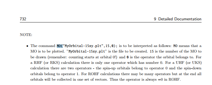
Я варьировала эти параметры, и в итоге, орбитали получились для (0,0) - (4,0) и для (0,1) - (4,1). Для остальных значений программа выдавала ошибки ERROR CODE RETURNED FROM PLOT PROGRAM или "Invalid MO requested for plot (<0 or >=DIM)".
Формы орбиталей (0,0) - (4,0) сохранились в файлах "H-0.cube" ... "H-4.cube". Их загрузили в PyMOL через функцию volume (так же, как и предыдущие орбитали):
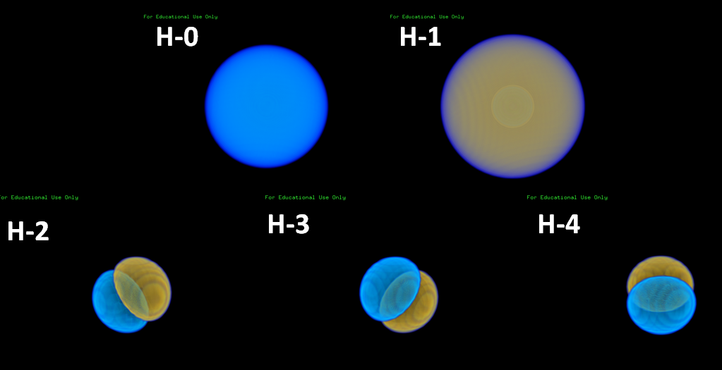
H-0 и H-1 это s-орбитали, остальные - p с разным числом m. Получается, что не вышло построить d-орбитали.
В итоге, при построении орбиталей с помощью orca орбитали более "гладкие", чем при построении вручную. Для сравнения нужно знать, какие орбитали orca каким уровням соответствуют.