Abstract

Klebsiella variicola is a species of bacteria which was originally identified as a benign endosymbiont in plants, but has since been associated with disease in humans, animals. Thus, research concerning the protein profile of this bacteria is essential for understanding its pathogenicity. This investigation characterized key genomic and proteomic features, determining: protein length distribution; the number of protein-coding and various RNA genes encoded on every replicon; genomic GC content; the distribution of intergenic gaps lengths; and the locations of the replication origin (oriC) and terminus (terC). Also, the comparison of K. variicola’s genome with different Klebsiella species was carried out.

1 Introduction

Klebsiella variicola was described as a species of Klebsielladistinct from its closely related species Klebsiella pneumoniae in 2004. Like other Klebsiella species, K.variicola is gram-negative, rod-shaped, non-motile, and covered by a polysaccharide capsule [1], [2].

KLebsiella variicola

Scientific classification [3]:

K. variicola is a versatile bacterium capable of colonizing different hosts such as plants, humans, insects and animals. Currently, K.variicola is gaining recognition as a cause of several human infections, especially bloodstream infections (BSIs) [4]. The research will examine the key features of K. variicola’s genome and proteome. Hopefully, the information studied will contribute to a more complex understanding of K. variicola’s biology and, especially, pathogenicity.

2 Methods

2.1 Information about genomic sequences, genome feature tables of K. variicola and other species considered it this research was obtained from NCBI, genomic sequences of chromosome and plasmids from NCBI Genome - GenBank assembly GCA_000019565.1. The genomic features table of K. variicola is available for downloading on NCBI Genome NCBI Genome . To obtain the features table the following steps were executed: 1) Using Bash command “wget” the compressed gunzip file “GCF_000019565.1_ASM1956v1_feature_table.txt.gz” was downloaded. 2) Using Bash command “gunzip” the received file was unpacked.

2.2 Standard information about the replicons, nucleotide composition of every replicon in K. variicola was obtained using python tools (see Supplementary materials/S1).

2.3 The counts of protein-coding genes and different RNA genes encoded by each K. variicola replicon were compiled using Google Sheets (see Supplementary materials/S2/sheet “per-replicons”). “COUNTIFS” function was utilized, it counts the number of values satisfying defined criteria. Furthermore, to determine the quantities of different rRNAs genes copies the following Bash command was executed: “cat *feature_table.txt | grep "^rRNA" | cut -f 14 | sort | uniq -c”, where “*feature_table.txt” — the genomic features table of K. variicola (see Methods/2.1). To determine the number of tRNAs for each amino acid the following Bash command was utilized: “cat *feature_table.txt | grep "^tRNA" | cut -f 14 | sort | uniq -c”, where “*feature_table.txt” — the genomic features table of K. variicola (see Methods/2.1).

2.4 The inter-CDS gaps length diagram was constructed using Google Sheets (see Supplementary materials/S2/sheet “interseq_lengths”). Primarily, inter-CDS gaps lengths were calculated: for the first and last CDS genes, the intergenic distance was calculated using the following formula: D = L - EL + SF - 1, where D – distance length, L – chromosome length, EL – last nucleotide position of last CDS (“end” column), SF – first nucleotide position of the first CDS (“start” column). For the remaining CDS, the gap length was derived using different formula: D = Sn+1 - En - 1, where D – distance length, Sn+1 – first nucleotide position of n+1 CDS, En – last position of n CDS. Next, histogram lengths intervals were chosen and the chart was generated. The “COUNTIFS” function was utilized to count the number of values that satisfy the intervals.

2.5 To determine the position of the origin (oriC) of replication and replication terminus (terC), GC-skew [5] and skewIT [6] methods were utilized. To generate the GC-skew and skewIT charts Genskew_cc (a commandline Genskew client) was used ("GitHub: https://github.com/univieCUBE/genskew") . The client software was obtained from its GitHub repository. All subsequent operations were performed in a terminal of an IDE (specifically, in this research JetBrains PyCharm was used). To access the usage instructions, the command «python3 -m genskew -h» was run. After that, two analyses were performed using the following commands on the sequence_chromosome.fasta file (K. variicola chromosome sequence): 1. python3 -m genskew -s 2000 -w 2000 -o jpg -n1 G -n2 C -d 300 -of /Users/user/Desktop ./sequence_chromosome.fasta — creates GC-skew plot 2. python3 -m genskew -s 2000 -w 2000 -o jpg -n1 G -n2 C -d 300 -of /Users/user/Desktop --skewIT true ./sequence_chromosome.fasta — creates skewIT plot.

2.6 A comparison table featuring main genomic differences between bacteria species within K. pneumoniae complex was made using python script (see Supplementary materials/S1) and Google Sheets (see Supplementary materials/S3/ sheet “CDS count”). CDS count was calculated with Google Sheets “COUNTIFS” methods, G/C content and chromosome length with the python script.

2.7 Protein length histogram was constructed in Google Sheets (see Supplementary materials/S4/sheet “Prot_length_hist”). Primarily, the lengths of every protein were found using following formula: L = (E - S)/3 - 1, where L – protein length, E - last nucleotide position of CDS, S – last nucleotide position of CDS. Then, the maximum and minimum protein sizes were identified using “MAX” and “MIN” functions respectively. Subsequently, the optimal bin length was determined and the “COUNTIFS” function was used to calculate the number of proteins contained within each bin. Next, the chart was constructed.

3 RESULTS and DISCUSSION

3.1 Main genomic features

Primarily, it is crucial to state that K. variicola has 3 replicons, two plasmids (pKP91 and pKP187) and a chromosome. The table below (Table 1) shows the standard information about the replicons:

Table 1. Standard replicon information.

Replicon	Size (bp)	GC content (%)
chromosome	5 641 239	57.29
pKP91	91 096	51.09
pKP187	187 922	47.15

Further researches gave more profound details (Table 2) about nucleotide composition in K. variicola genome:

Table 2. Nucleotide composition of replicons.

Replicon	A	T	G	C
Chromosome	1203247	1206346	1612759	1618887
	21.33%	21.38%	28.59%	28.7%
pKP91	22441	22112	23676	22867
	24.63%	24.27%	25.99%	25.1%
pKP187	49794	49520	44794	43814
	26.5%	26.35%	23.84%	23.31%

As the table shows, Chargaff’s rules apply for analyzed replicons [7].

3.2 Replicon composition

Furthermore, the amount of genes encoding proteins and different types of RNA per every replicon was counted (Table 3):

Table 3. Number of Protein-Coding and RNA Genes per Replicon

Replicon	Chromosome	pKP91	pKP187
Cds with protein	5254	89	165
rRNA	25	0	0
tRNA	88	0	0
tmRNA	1	0	0
antisense RNA	2	0	0
ncRNA	11	0	0
pseudogene	108	12	25

It is obvious that the vast majority of genes responsible for ensuring vital activity are encoded on the chromosome: A total of 5254 proteins are encoded, 88 t-RNA genes, 25 rRNA genes and some minor types RNA genes are present.

It is reasonable to assume that there are significantly more than 3 rRNA genes, because they are assembled into clusters (is often referred to as rDNA) of several copies encoding one of the three rRNAs: 8 copies of 16s, 8 copies of 23s and 9 copies of 5s. The rRNA genes form clusters containing multiple copies in order to increase the synthesis of rRNA and, eventually, ribosome formation [8].

Moreover, It should be noted that there are relatively many t-RNA genes in the genome. Usually, their number does not exceed 61, since there are 61 possible coding codons in total (4 3 - 3 stop codons). But most organisms possess significantly fewer than 61 distinct tRNAs. This is possible due to the flexibility in codon-anticodon pairing described by the wobble rules. A wobble base pair is a pairing between two nucleotides in RNA molecules that does not follow Watson–Crick base pair rules. The four main wobble base pairs are guanine-uracil (G–U), hypoxanthine–uracil (I–U), hypoxanthine–adenine (I–A), and hypoxanthine–cytosine (I–C) [9]. The Bacterial Genetic Code (Translation Table 11) is characteristic to K. variicola [10]. This translation table is identical to the Standard Genetic Code [11] with one known exception: in some bacteria, such as E. coli and Bacillus subtilis, the canonical stop codon “UGA” can encode tryptophan. However, this “UGA-Trp” reassignment is not characteristic to K. variicola. Table 4 presents the codon count per amino acid for translation table 11 and the tRNA gene count for each amino acid in K. variicola genome.

As shown in Table 4, the number of tRNA genes in the genome exceeds the number of corresponding codons for the majority of amino acids (13 out of 20). The inverse is true for cysteine (Cys), histidine (His), proline (Pro), and serine (Ser), where the codon count is greater than the tRNA gene count. Tryptophan (Trp), threonine (Thr), and phenylalanine (Phe) represent an equilibrium case, with equal numbers of codons and tRNA genes.

Furthermore, analysis of the tRNA repertoire revealed the presence of a selenocysteine-specific tRNA. This finding indicates that K. variicola utilizes selenocysteine (Sec), suggesting that its proteome likely includes selenoproteins [12].

There is a lack of information about plasmids pKP91 and pKP187 in K. variicola. Here is information about plasmids pKP187 and pKP91 from the related bacterium Klebsiella pneumoniae 342: pKP187 plasmid encodes proteins involved in replication, partitioning/maintenance, arsenate and tellurite resistance, also some regions of pKP187 consist of genes taking part in carbohydrate metabolism. pKP91 plasmid encodes a putative fusaric acid resistance gene as well as several oxidoreductase genes [13].

3.3 Inter-CDs distances

The intergenic distances between cds on the “+” strand were calculated, and a histogram was constructed based on the obtained data (Fig. 1.):

It is important to clarify that the defined intergenic gaps contain no CDS on the “+” strand but may contain features on the complementary strand, including reverse-strand CDS and RNA genes. The proteome analysis in section 3.6 indicates a high frequency of proteins with the length ≥50 amino acids. Consequently, many gaps exceeding 200 nucleotides in length (calculated as: 50 codons * 3 nucleotides + 3 for a stop codon + ~50 for regulatory sequences) are likely to harbor CDS on the “-” strand.To better assess genomic coding density, a histogram of intergenic gap lengths (FIg. 2.) was constructed, accounting for coding sequences on both the “+” and “-” strands:

Analysis of the presented diagram demonstrates high-density gene packing. The vast majority of intergenic intervals do not exceed 200–250 bp. Additionally, 807 instances of coding sequence (CDS) overlap were detected. This pattern is consistent with and can be explained by the operon-based organization of bacterial genomes [14]. Bacteria and archaea typically possess small genomes that are tightly packed with protein-coding genes. The compactness of prokaryotic genomes is commonly perceived as evidence of adaptive genome streamlining caused by strong purifying selection in large microbial populations. In such populations, even the small cost incurred by nonfunctional DNA because of extra energy and time expenditure is thought to be sufficient for this extra genetic material to be eliminated by selection [15].

3.4 Localization of the origin and terminus of replication.

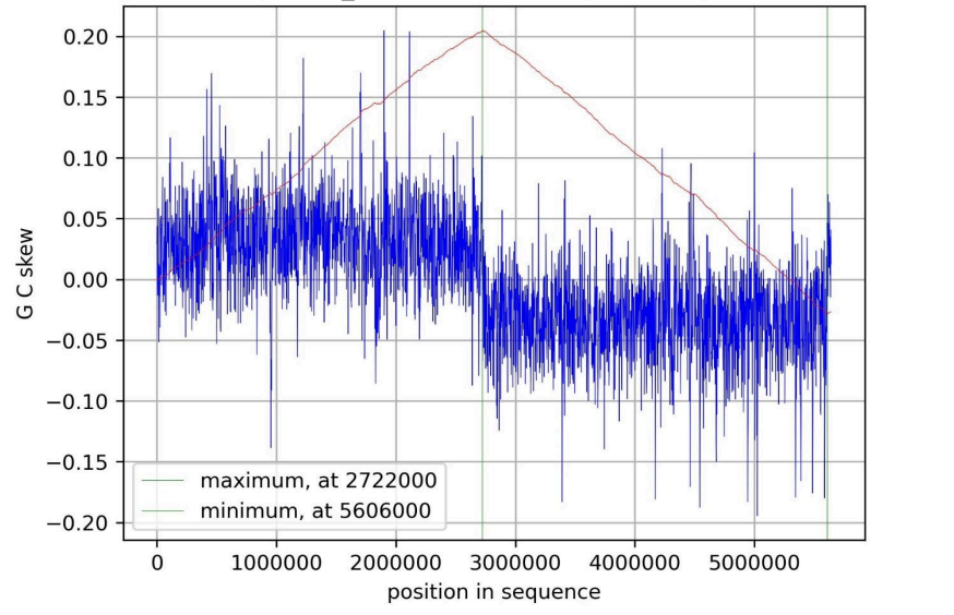
The positions of the putative origin and terminus of replication were identified using the cumulative GC skew method (Fig. 3.):

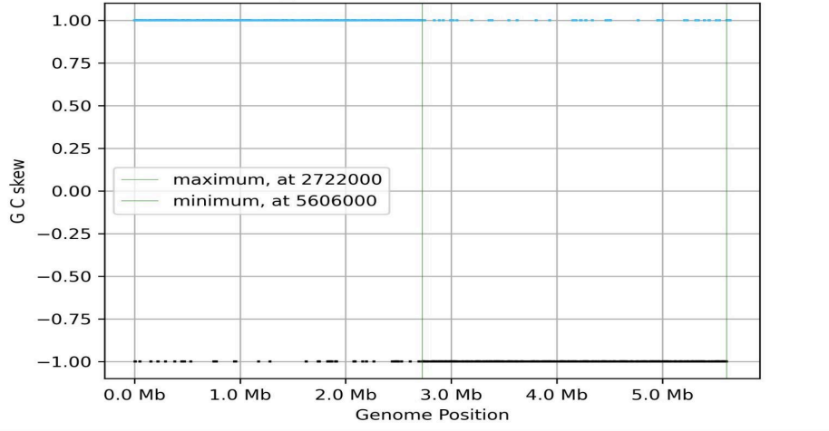
The cumulative GC skew analysis revealed a characteristic sawtooth pattern across the circular chromosome of K.variicola. A global minimum in the cumulative skew profile was identified at position 5606000 bp, marking the predicted origin of replication (oriC). Conversely, a global maximum was observed at approximately 2722000 bp, corresponding to the replication terminus (terC). The skewIT plot was also created (Fig. 4.):

The skewIT analysis identifies the window of maximal skewness, thereby delineating the boundary between the A and B partitions. The position of this boundary (2722000 bp) corresponds to the terminus of replication (terC). And the window of minimal skewness indicates the approximate location of the replication origin (oriC) near bp 5606000 (see Methods, section 2.6). Thus, the skewIT analysis confirmed and refined the predicted locations of oriC and terC.

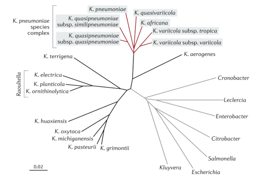
3.5. Comparison of K. variicola genome with different

The Klebsiella pneumoniae complex (Fig. 5.) includes seven similar species: K. pneumoniae subsp. pneumoniae, K. quasipneumoniae subsp. quasipneumoniae, K. quasipneumoniae subsp. similipneumoniae, K. quasivariicola, K. africana, K. variicola subsp. tropica and K. variicola subsp. variicola (subsp. variicola is often referred to as “K. variicola” ) [16].

The table below (Table 5) provides some information about K. pneumoniae complex species chromosomes:

Table 5. Genomic features of K. pneumoniae complex species.

Species	Chromosome length (bp)	G/C content (%)	CDS count
K. variicola	5 641 239	57,29	5653
K. quasipneumoniae subsp. quasipneumoniae	5 343 479	58,14	5177
K. pneumoniae	5 333 941	57,48	5779
K. africana	5 243 981	57,16	5129
K. quasipneumoniae subsp. similipneumoniae	5 395 457	57,68	5507
K. variicola subsp. tropica	5 607 968	57,17	5632
K. quasivariicola	5 489 214	57,16	5396

Due to substantial overlap in their biochemical and phenotypic profiles, these species cannot be reliably differentiated by traditional microbiological methods. This taxonomic ambiguity, particularly the frequent misidentification of K. variicola, has hindered research into its unique biology and obscured its distinct clinical implications [17]. Significant attempts are now being made across the scientific community to discover the best strategies for distinguishing between those species.

3.6. Protein profile

Fundamental research concerning the protein distribution based on their length was conducted. The histogram below (Fig. 6.) illustrates the length distribution of proteins found in K.variicola:

Fig. 6. Protein length distribution in K. variicola.

According to the diagram, the K.variicola’s proteome consists mostly of relatively small proteins, approximately 75 percent of proteins have a length of 0 - 400 amino acid residues. Which refers to the fact that most of the proteins either structurally consist of small amount of domains or exist as monomers, as it is usual in prokaryotes [18].