Optimal pairwise alignment

Last updated: 26-04-2017.

Files to download

Task 1. Global and local alignment comparison

Alignments for the first task were received using Emboss programs 'needle' and 'water'. Main information about them is presented in Table 1, alignments themselves are presented in Figures 1 and 2. Global alignment length is 658, local one is 612. So, local alignment is shorter than global one. Main differences betwixt global and local alignments are in algorithms themselves which are discussed in tasks 4 and 5. Global alignment suggests that observed sequences are homologous along the entire length, local alignment admits that proteins may contain non-homologous plots just as homologous ones. Using figures one and two it is not hard to notice, that global and local alignments of HS71L_MOUSE (P16627) and DNAK_METBF (Q465Y6) are almost absolutely the same: local alignment is a global one without 1..10 positions.

Figure 1. Global alignment of HS71L_MOUSE (P16627) and DNAK_METBF (Q465Y6).

Figure 2. Local alignment of HS71L_MOUSE (P16627) and DNAK_METBF (Q465Y6).

Sequence name	AC	Alignment type	Sequence length	Alignment length	Amount of conservative residues	Percent of conservative residues	Amount of functional-conservative residues	Percent of functional-conservative residues	Amount of gaps	Percent of gaps	Amount indels
Homologous sequences
HS71L_MOUSE/1-641	P16627	GLOBAL	641	658	290	44,1 %	406	61,7 %	13	2,0 %	5
DNAK_METBF/1-620	Q465Y6	GLOBAL	620	658	290	44,1 %	406	61,7 %	38	5,8 %	8
HS71L_MOUSE/1-641	P16627	LOCAL	606	612	282	46,1 %	396	64,7 %	6	1,0 %	2
DNAK_METBF/1-620	Q465Y6	LOCAL	574	612	282	46,1 %	396	64,7 %	38	6,2 %	8
Non-homologous sequences
1
MALE_SALTY	P19576	LOCAL	312	379	77	20,3 %	127	33,5 %	67	17,7 %	16
PLED_CAUCN	B8GZM2	LOCAL	316	379	77	20,3 %	127	33,5 %	63	16,6 %	9
2
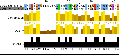
MALE_SALTY	P19576	LOCAL	42	42	11	26,2 %	21	50,0 %	0	0,0 %	0
FMM1_NEIGO	P02974	LOCAL	35	42	11	26,2 %	21	50,0 %	7	1,7 %	1
3
MALE_SALTY	P19576	LOCAL	98	118	25	21,2 %	39	33,1 %	20	17,0 %	3
Y2262_MYCBO	P65689	LOCAL	92	118	25	21,2 %	39	33,1 %	26	22,0 %	5
4
MALE_SALTY	P19576	LOCAL	94	147	35	23,8 %	54	36,7 %	53	36,1 %	6
HETS_PODAS	Q03689	LOCAL	140	147	35	23,8 %	54	36,7 %	7	4,8 %	3
5
MALE_SALTY	P19576	LOCAL	331	386	79	20,5 %	131	44,0 %	55	14,3 %	11
A0A126V644_9RHOB	A0A126V644	LOCAL	312	386	79	20,5 %	131	44,0 %	74	19,2 %	12

Table 1. Some information about observed alignments.

Attribute	Global	Local
Score matrix	BLOSUM62	BLOSUM62
Indel opening penalty	10	10
Indel extension penalty	0,5	0,5
End gap penalty applying	No	-
End gap opening penalty	10	-
End gap extending penalty	0,5	-

Table 2. Alignment parameters.

Task 2. Local alignment of homologous and non-homologous sequences comparison

According to Table 1, Figures 2 and 3, local alignments of non-homologous sequences are most likely shorter than alignments of homologous sequences. Also, they have less percent of conservative and functional-conservative residues. Talking about biological sense, local alignment of non-homologous sequences seems senseless and not informative at all: local alignment algorithm is suitable for aligning homologous domain proteins.

Figure 3. Example of two non-homologous sequences alignment.

Task 3. Multiple, local and global alignments comparison

HS71L_MOUSE (P16627) and DNAK_METBF (Q465Y6) sequences were chosen for this task. All alignments are seem similar but there is a couple of differences betwixt them, for example: in multiple alignment VAL(80) stands against TYR(109), in local and global alignments VAL(80) stands against VAL(107); in multiple alignment THR(81) stands against LYS(110), in local and global alignments THR(81) stands against SER(108); in multiple alignment LEU(82) stands against GLY(111), in local and global alignments LEU(82) stands against TYR(109). Most of differences are located in the beginning and the end of sequences.

Figure 4. Multiple, local and global alignments comparison.

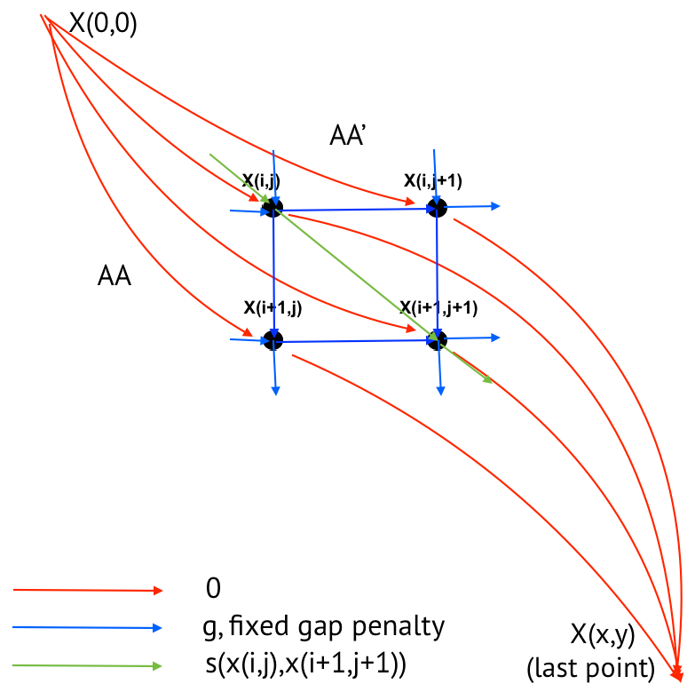
Task 4. Global alignment with affine penalties graph

Graph of global alignment with affine penalties is presented in Figure 5.

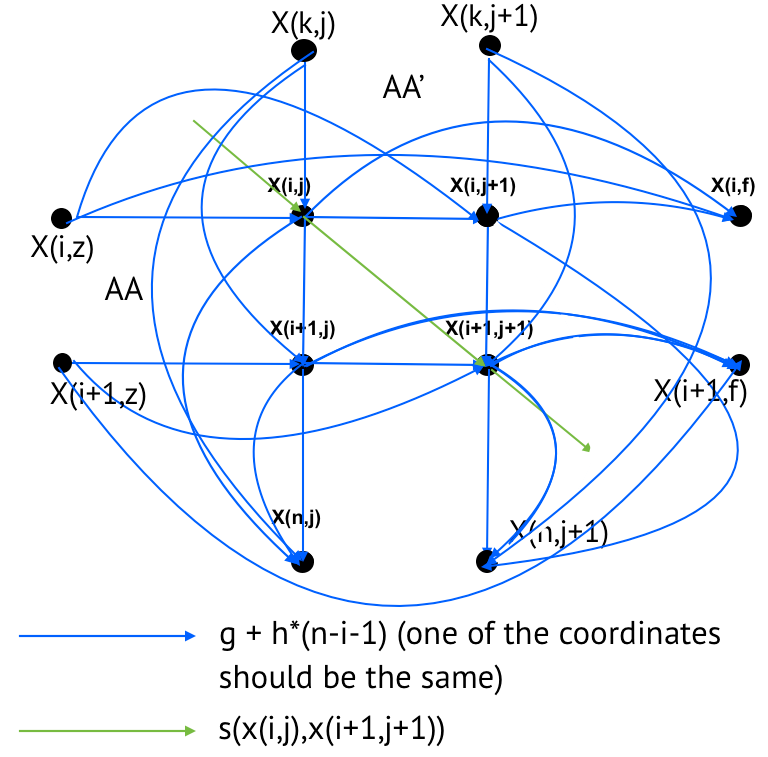
Figure 5. Global alignment with affine penalties graph.

Task 5. Local alignment with linear penalties graph

Graph of local alignment with linear penalties is presented in Figure 6.

Figure 6. Local alignment with linear penalties graph.

Task 6. "Scores of friendliness"

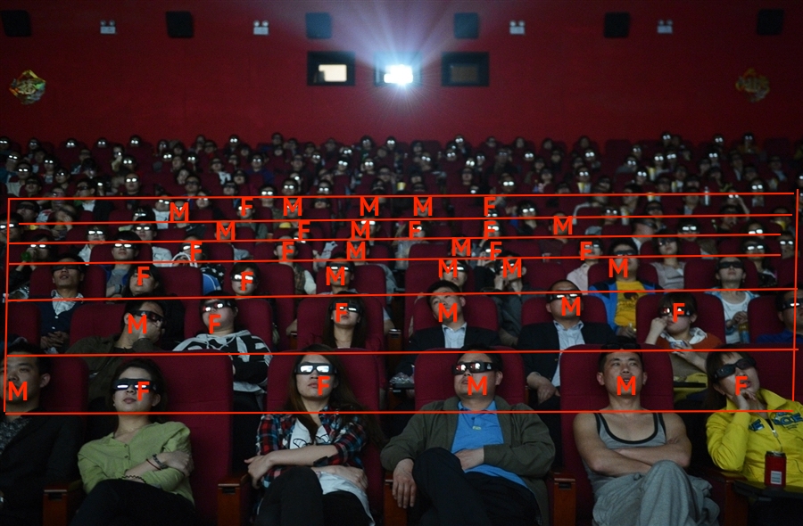
Seat scheme is presented in Figure 7 and Insertion 1. The probability of meeting a male q(M) is 0.53, female q(F) is 0.47. Amount of pairs is 6*5 = 30. If the audience seated casually and independently of each other, then there is q(M)*q(M)*30 = 8.4 of MM pairs, 6.6 FF pairs, 7.4 pairs of FM and MF. Actual shares of pairs is: p(MM) = 0.27, p(FF) = 0.2 p(FM) = 0.27. The inclination of men to sit next to each other L(MM) is p(MM)/q(M)*q(M), similarly for other pairs. For example, -100*log_2(L(MM)) is called male-male score of friendliness. Table of scores of friendliness has number 3.

MFMMMF
MFMFFM
FFMMFF
FFMMMM
MFFMMF
MFFMMF

Insertion 1. Seat scheme.

	M	F	Sum
M	496	478	974
F	478	504	982
Sum	974	982

Table 3. Scores of friendliness